Puppet Extension Points - part 2
After the first part in this series of article on Puppet extensions points, I’m proud to deliver a new episode focusing on Types and Providers. Note that th...
After the first part in this series of article on Puppet extensions points, I’m proud to deliver a new episode focusing on Types and Providers. Note that th...
It’s been a long time since my last blog post, almost a year. Not that I stopped hacking on Puppet or other things (even though I’m not as productive as I ha...
It’s been a long time since my last puppet blog post about file content offloading. Two puppetcamps even passed (more on the last one in a next blog article)...
The Days of Wonder News Center is running Wordpress which until a couple of days used Gengo for multilingual stuff. Back when we started using Wordpress for ...
Puppet really shines at configuration management, but there are some things it is not good at, for instance file sourcing of large files, or managing deep hi...
As every reader of this blog certainly know, I’m a big fan of Puppet, using it in production on Days of Wonder servers, up to the point I used to contribute ...
I’m really proud to announce the release of the version 1.0 of mysql-snmp. What is mysql-snmp? mysql-snmp is a mix between the excellent MySQL Cacti Templa...
Yes, I know… I released v0.7 less than a month ago. But this release was crippled by a crash that could happen at start or reload. Changes Bonus in this ne...
I’m proud to announce the release of Nginx Upload Progress module v0.7 This version sees a crash fix and various new features implemented by Valery Kholodko...
At Days of Wonder we are huge fans of MySQL (and since about a year of the various Open Query, Percona, Google or other community patches), up to the point w...
This morning I got the joy to see that my Puppet Camp 2009 slides had been selected by Slideshare to appear on their home page:
I attended Puppet Camp 2009 in San Francisco last week. It was a wonderful event and I could meet a lot of really smart developers and sysadmins from a lot o...
This week on #puppet, Nico asked for a storeconfigs live example. So I thought, a blog post would be perfect to post an example of a storeconfigs use case an...
As a Puppet Mongrel Nginx user, I’m really ashamed about the convoluted nginx configuration needed (two server blocks listening on different ports, you need ...
It’s been a long time since my last post… which just means I was really busy both privately, on the Puppet side and at work (I’ll talk about the Puppet side ...
As announced in my last edit of my yesterday post Puppet and JRuby a love and hate story, I finally managed to run a webrick puppetmaster under JRuby with a ...
Since I heard about JRuby about a year ago, I wanted to try to run my favorite ruby program on it. I’m working with Java almost all day long, so I know for s...
Note: when I started writing this post, I didn’t know it would be this long. I decided then to split it in several posts, each one covering one or more inter...
Thanks to Days of Wonder the company I work for, I’m proud to release in Free Software (GPL):
There is something I used to hate to do. And I think all admins also hate to do that.
When I wrote my previous post titled all about storedconfigs, I was pretty confident I explained everything I could about storedconfigs… I was wrong of cours...
Since a long time people (including me) complained that storeconfigs was a real resource hog. Unfortunately for us, this option is so cool and useful.
This seems to be recurrent this last 3 or 4 days with a few #puppet, redmine or puppet-user requests, asking about why puppetd is consuming so much CPU an...
In the Days of Wonder Paris Office (where is located our graphic studio, and incidentally where I work), we are using Bacula to perform the multi-terabyte ...
Yesterday we had the February Puppet Dev Call with unfortunately poor audio, lots of Skype disconnections which for a non native English speaker like me re...
If you like me are struggling with old disks (in my case SCSI 10k RPM Ultra Wide 2 HP disks) that exhibits bad blocks, here is a short survival howto.
From time to time we get some complaints about so-called Puppet memory leaks either on #puppet, on the puppet-user list or in the Puppet redmine.
Have you ever wondered why net-snmp doesn’t report a ccomments: true orrect interface speed on Linux?
Since a few months we are monitoring our infrastructure at Days of Wonder with OpenNMS. Until this afternoon we were running the beta/final candidate versio...
As more or less promised in my series of post about Puppet Extension Points, here is the first post about Puppet Internals.
This article is a follow-up of those previous two articles of this series on Puppet Internals:
After the first part in this series of article on Puppet extensions points, I’m proud to deliver a new episode focusing on Types and Providers. Note that th...
It’s been a long time since my last blog post, almost a year. Not that I stopped hacking on Puppet or other things (even though I’m not as productive as I ha...
The puppet-users or #puppet freenode irc channel is full of questions or people struggling about the puppet SSL PKI. To my despair, there are also people wan...
It’s been a long time since my last puppet blog post about file content offloading. Two puppetcamps even passed (more on the last one in a next blog article)...
Puppet really shines at configuration management, but there are some things it is not good at, for instance file sourcing of large files, or managing deep hi...
As every reader of this blog certainly know, I’m a big fan of Puppet, using it in production on Days of Wonder servers, up to the point I used to contribute ...
This morning I got the joy to see that my Puppet Camp 2009 slides had been selected by Slideshare to appear on their home page:
I attended Puppet Camp 2009 in San Francisco last week. It was a wonderful event and I could meet a lot of really smart developers and sysadmins from a lot o...
This week on #puppet, Nico asked for a storeconfigs live example. So I thought, a blog post would be perfect to post an example of a storeconfigs use case an...
As usual, I’m faster to create things than to talk about them.
As a Puppet Mongrel Nginx user, I’m really ashamed about the convoluted nginx configuration needed (two server blocks listening on different ports, you need ...
As announced in my last edit of my yesterday post Puppet and JRuby a love and hate story, I finally managed to run a webrick puppetmaster under JRuby with a ...
Since I heard about JRuby about a year ago, I wanted to try to run my favorite ruby program on it. I’m working with Java almost all day long, so I know for s...
When I wrote my previous post titled all about storedconfigs, I was pretty confident I explained everything I could about storedconfigs… I was wrong of cours...
Since a long time people (including me) complained that storeconfigs was a real resource hog. Unfortunately for us, this option is so cool and useful.
This seems to be recurrent this last 3 or 4 days with a few #puppet, redmine or puppet-user requests, asking about why puppetd is consuming so much CPU an...
Yesterday we had the February Puppet Dev Call with unfortunately poor audio, lots of Skype disconnections which for a non native English speaker like me re...
From time to time we get some complaints about so-called Puppet memory leaks either on #puppet, on the puppet-user list or in the Puppet redmine.
Puppet really shines at configuration management, but there are some things it is not good at, for instance file sourcing of large files, or managing deep hi...
As every reader of this blog certainly know, I’m a big fan of Puppet, using it in production on Days of Wonder servers, up to the point I used to contribute ...
I’m really proud to announce the release of the version 1.0 of mysql-snmp. What is mysql-snmp? mysql-snmp is a mix between the excellent MySQL Cacti Templa...
Yes, I know… I released v0.7 less than a month ago. But this release was crippled by a crash that could happen at start or reload. Changes Bonus in this ne...
I’m proud to announce the release of Nginx Upload Progress module v0.7 This version sees a crash fix and various new features implemented by Valery Kholodko...
I attended Puppet Camp 2009 in San Francisco last week. It was a wonderful event and I could meet a lot of really smart developers and sysadmins from a lot o...
As a Puppet Mongrel Nginx user, I’m really ashamed about the convoluted nginx configuration needed (two server blocks listening on different ports, you need ...
It’s been a long time since my last post… which just means I was really busy both privately, on the Puppet side and at work (I’ll talk about the Puppet side ...
As announced in my last edit of my yesterday post Puppet and JRuby a love and hate story, I finally managed to run a webrick puppetmaster under JRuby with a ...
Since I heard about JRuby about a year ago, I wanted to try to run my favorite ruby program on it. I’m working with Java almost all day long, so I know for s...
Since a long time people (including me) complained that storeconfigs was a real resource hog. Unfortunately for us, this option is so cool and useful.
Yesterday we had the February Puppet Dev Call with unfortunately poor audio, lots of Skype disconnections which for a non native English speaker like me re...
From time to time we get some complaints about so-called Puppet memory leaks either on #puppet, on the puppet-user list or in the Puppet redmine.
I like them refreshing, of course:
After the first part in this series of article on Puppet extensions points, I’m proud to deliver a new episode focusing on Types and Providers. Note that th...
It’s been a long time since my last blog post, almost a year. Not that I stopped hacking on Puppet or other things (even though I’m not as productive as I ha...
Puppet really shines at configuration management, but there are some things it is not good at, for instance file sourcing of large files, or managing deep hi...
As every reader of this blog certainly know, I’m a big fan of Puppet, using it in production on Days of Wonder servers, up to the point I used to contribute ...
I attended Puppet Camp 2009 in San Francisco last week. It was a wonderful event and I could meet a lot of really smart developers and sysadmins from a lot o...
As announced in my last edit of my yesterday post Puppet and JRuby a love and hate story, I finally managed to run a webrick puppetmaster under JRuby with a ...
Since I heard about JRuby about a year ago, I wanted to try to run my favorite ruby program on it. I’m working with Java almost all day long, so I know for s...
Since a long time people (including me) complained that storeconfigs was a real resource hog. Unfortunately for us, this option is so cool and useful.
From time to time we get some complaints about so-called Puppet memory leaks either on #puppet, on the puppet-user list or in the Puppet redmine.
I’m really proud to announce the release of the version 1.0 of mysql-snmp. What is mysql-snmp? mysql-snmp is a mix between the excellent MySQL Cacti Templa...
At Days of Wonder we are huge fans of MySQL (and since about a year of the various Open Query, Percona, Google or other community patches), up to the point w...
Thanks to Days of Wonder the company I work for, I’m proud to release in Free Software (GPL):
When I wrote my previous post titled all about storedconfigs, I was pretty confident I explained everything I could about storedconfigs… I was wrong of cours...
Since a long time people (including me) complained that storeconfigs was a real resource hog. Unfortunately for us, this option is so cool and useful.
Since a few months we are monitoring our infrastructure at Days of Wonder with OpenNMS. Until this afternoon we were running the beta/final candidate versio...
Puppet really shines at configuration management, but there are some things it is not good at, for instance file sourcing of large files, or managing deep hi...
As every reader of this blog certainly know, I’m a big fan of Puppet, using it in production on Days of Wonder servers, up to the point I used to contribute ...
Yes, I know… I released v0.7 less than a month ago. But this release was crippled by a crash that could happen at start or reload. Changes Bonus in this ne...
I’m proud to announce the release of Nginx Upload Progress module v0.7 This version sees a crash fix and various new features implemented by Valery Kholodko...
As a Puppet Mongrel Nginx user, I’m really ashamed about the convoluted nginx configuration needed (two server blocks listening on different ports, you need ...
It’s been a long time since my last post… which just means I was really busy both privately, on the Puppet side and at work (I’ll talk about the Puppet side ...
Welcome to the 4th episode of this series of articles about designing a full keyboard from scratch. So far we’ve seen:
Welcome for the third episode of this series of posts about designing a full fledged keyboard from scratch. The first episode focused on the electronic schem...
In the handwired build log part 1 we saw a technique to build a nice keyboard matrix without using a PCB.
Update 1: I’ve finished the second part of the serie
The same way I created mysql-snmp a small Net-SNMP subagent that allows exporting performance data from MySQL through SNMP, I’m proud to announce the first r...
I’m really proud to announce the release of the version 1.0 of mysql-snmp. What is mysql-snmp? mysql-snmp is a mix between the excellent MySQL Cacti Templa...
Thanks to Days of Wonder the company I work for, I’m proud to release in Free Software (GPL):
This seems to be recurrent this last 3 or 4 days with a few #puppet, redmine or puppet-user requests, asking about why puppetd is consuming so much CPU an...
Since a few months we are monitoring our infrastructure at Days of Wonder with OpenNMS. Until this afternoon we were running the beta/final candidate versio...
The Days of Wonder News Center is running Wordpress which until a couple of days used Gengo for multilingual stuff. Back when we started using Wordpress for ...
At Days of Wonder we are huge fans of MySQL (and since about a year of the various Open Query, Percona, Google or other community patches), up to the point w...
There is something I used to hate to do. And I think all admins also hate to do that.
In the Days of Wonder Paris Office (where is located our graphic studio, and incidentally where I work), we are using Bacula to perform the multi-terabyte ...
If you like me are struggling with old disks (in my case SCSI 10k RPM Ultra Wide 2 HP disks) that exhibits bad blocks, here is a short survival howto.
All started a handful of months ago, when it appeared that we’d need to build some of our native software on Windows. Before that time, all our desktop softw...
So I know this blog has been almost abandoned, but that’s not because I don’t have anything to say. At contrary, I’ve never dealt with so many different tool...
Paris is more and more becoming the DevOps place to be. We (apparently) successfully rebooted the Paris DevOps Meetups, with already two events so far, and t...
Welcome on my blog for this new Year. After writing an answer to a thread regarding monitoring and log monitoring on the Paris devops mailing list, I thought...
After seeing @KrisBuytaert tweet a couple of days ago about offering priority registration for the upcoming Devopsdays Roma next October to people blogging a...
I’m really proud to announce the release of the version 1.0 of mysql-snmp. What is mysql-snmp? mysql-snmp is a mix between the excellent MySQL Cacti Templa...
Thanks to Days of Wonder the company I work for, I’m proud to release in Free Software (GPL):
Have you ever wondered why net-snmp doesn’t report a ccomments: true orrect interface speed on Linux?
As announced in my last edit of my yesterday post Puppet and JRuby a love and hate story, I finally managed to run a webrick puppetmaster under JRuby with a ...
Since I heard about JRuby about a year ago, I wanted to try to run my favorite ruby program on it. I’m working with Java almost all day long, so I know for s...
I like them refreshing, of course:
All started a handful of months ago, when it appeared that we’d need to build some of our native software on Windows. Before that time, all our desktop softw...
And I’m now proud to present the second installation of my series of post about Puppet Internals:
I decided this week-end to try the more popular puppet master stacks and benchmark them with puppet-load (which is a tool I wrote to simulate concurrent clie...
As announced in my last edit of my yesterday post Puppet and JRuby a love and hate story, I finally managed to run a webrick puppetmaster under JRuby with a ...
Hi,Welcome to my personal blog!
It’s a long time since I blogged about photography, but I’m coming back from 2 weeks vacation in Sicily armed with my Nikon D700, so it’s the perfect time to...
If you had a look to my About Me page, you know that one of my hobby is photography. Until a couple of weeks ago, I was still doing analog photography with ...
Yes, I know… I released v0.7 less than a month ago. But this release was crippled by a crash that could happen at start or reload. Changes Bonus in this ne...
I’m proud to announce the release of Nginx Upload Progress module v0.7 This version sees a crash fix and various new features implemented by Valery Kholodko...
The same way I created mysql-snmp a small Net-SNMP subagent that allows exporting performance data from MySQL through SNMP, I’m proud to announce the first r...
This article is a follow-up of those previous two articles of this series on Puppet Internals:
I like them refreshing, of course:
You certainly know that I work for the boardgame publisher Days of Wonder, and we announced a couple of days ago our new boardgame Small World:
Note: when I started writing this post, I didn’t know it would be this long. I decided then to split it in several posts, each one covering one or more inter...
It’s been a long time since my last post… which just means I was really busy both privately, on the Puppet side and at work (I’ll talk about the Puppet side ...
I’m really proud to announce the release of the version 1.0 of mysql-snmp. What is mysql-snmp? mysql-snmp is a mix between the excellent MySQL Cacti Templa...
The Days of Wonder News Center is running Wordpress which until a couple of days used Gengo for multilingual stuff. Back when we started using Wordpress for ...
The Days of Wonder News Center is running Wordpress which until a couple of days used Gengo for multilingual stuff. Back when we started using Wordpress for ...
The puppet-users or #puppet freenode irc channel is full of questions or people struggling about the puppet SSL PKI. To my despair, there are also people wan...
The puppet-users or #puppet freenode irc channel is full of questions or people struggling about the puppet SSL PKI. To my despair, there are also people wan...
At Days of Wonder we develop several Java projects (for instance our online game servers). Those are built with Maven, and most if not all are using Google P...
At Days of Wonder we develop several Java projects (for instance our online game servers). Those are built with Maven, and most if not all are using Google P...
At Days of Wonder we develop several Java projects (for instance our online game servers). Those are built with Maven, and most if not all are using Google P...
All started a handful of months ago, when it appeared that we’d need to build some of our native software on Windows. Before that time, all our desktop softw...
Welcome to the 4th episode of this series of articles about designing a full keyboard from scratch. So far we’ve seen:
I’ll now cover:
This is again a long episode that took quite long time to write, sorry for the wait. Feel free to leave a comment if you have any questions or find anything suspect :)
We need to export our PCB out of Kicad and send it to the factory. Hopefully, all the factories out there use a common file format that is called the Gerber format.
This file format is a vectorial format that describe precisely the layer traces and zones, silk screens, and sometimes where to drill holes (some manufacturer require Excellon format). This has become a kind of interchange standard for PCB factories. This is an old file format that was used to send numerical commands to Gerber plotters in the 70s. Since then the format has evolved and we’re dealing now with Extended Gerber files.
Back to my PCB, I can generate my set of Gerber files to be sent to the factory from pcbnew by going to File → Plot…. A new window opens where I can configure the output.
The options to set will depend on the manufacturer. Here’s a few manufacturer Kicad recommandations and settings:
Caution: different manufacturer have different tolerances and capabilities (for instance minimum track size, via size, board size, etc). Make sure you check with them if your PCB can be manufactured.
This time, I’m going to be using JLCPCB. Here’s the recommended setup for JLCPCB with Kicad 5.1:
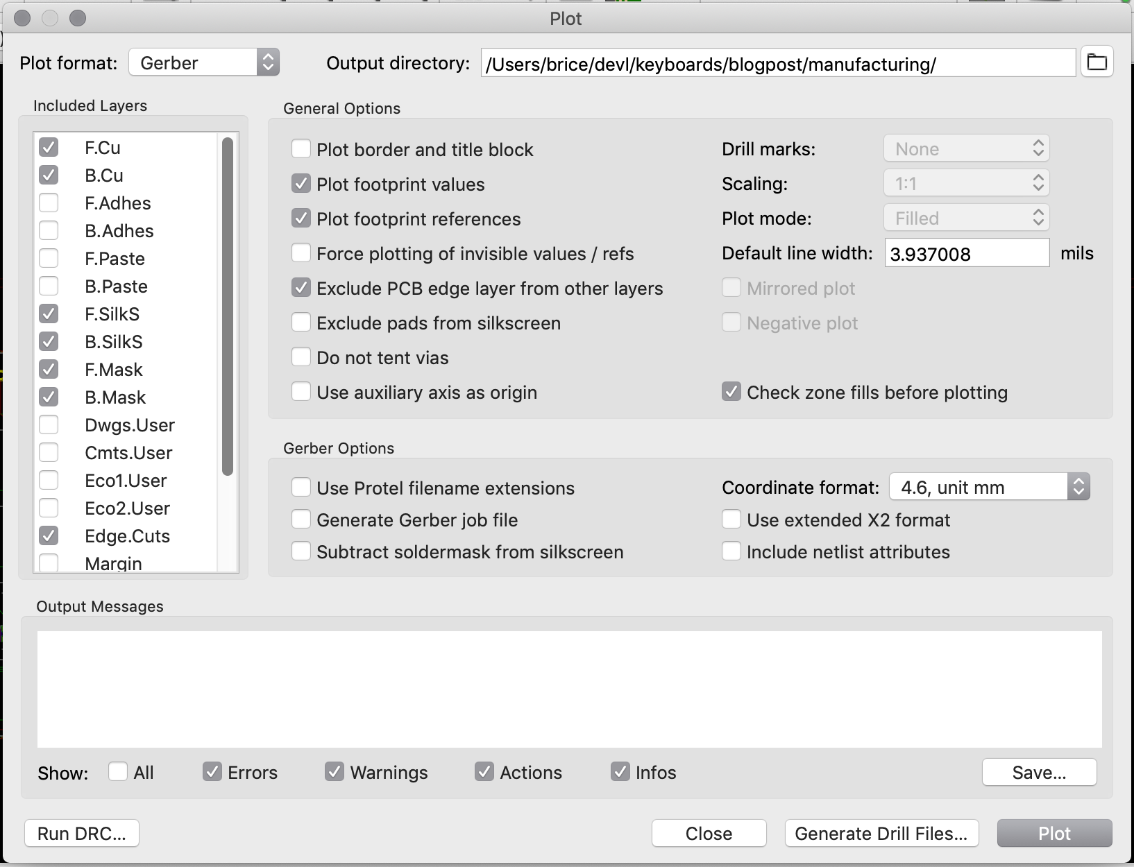
For this project the following layers needs to be checked:
F.CuB.CuF.SilkSB.SilkSF.MaskB.MaskEdge.CutsThe first two are for drawing the tracks and pads, the two next ones are the components reference and value indications (and the art), the two mask layers contains the zone where the copper layers will be seen (ie pads and holes), and finally the Edge.Cuts layer contains the board outline.
Make sure the chosen format is Gerber, then choose a sensible output folder (I like to put those files in a manufacturing subfolder of my PCB repository).
And additionnally those options need to be checked:
When clicking on the Plot button, the files are generated (in the folder previously entered).
The next step is to generate the drill files, which contain the location where to drill holes (for both types of holes: mounting holes or for through-hole components, and for plated and non-plated holes). This can be done by clicking on the Generate Drill Files button next to the Plot button in the previous window:
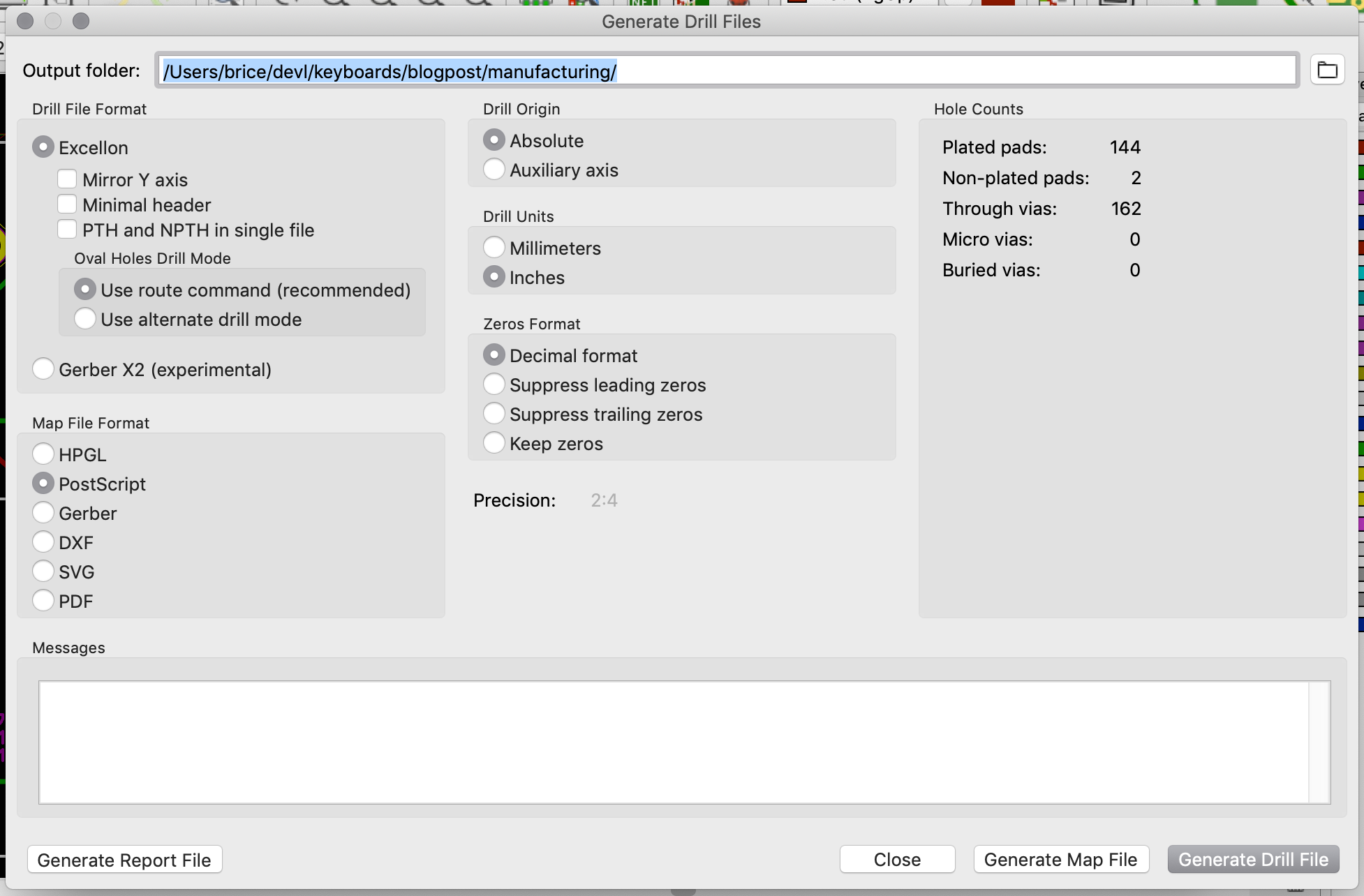
The important options to check are:
Generating the drill file is done by clicking on the Generate Drill File (oh that was unexpected :) )
This produces two new files in my manufacturing folder, one for the plated holes and the other ones for the non-plated holes. The manufacturing folder now contains:
aek67-B_Cu.gbraek67-B_Mask.gbraek67-B_SilkS.gbraek67-Edge_Cuts.gbraek67-F_Cu.gbraek67-F_Mask.gbraek67-F_SilkS.gbraek67-NPTH.drlaek67-PTH.drlNow zip everything (cd manufacturing ; zip -r pcb.zip * if you like the command-line). That’s what we’re going to upload to the manufacturer.
If you’re interested in PCB manufacturing, you can watch this video of the JLCPCB factory, you’ll learn a ton of things about how PCB are made these days.
So, the process is to upload the Gerber and drill files to the factory. But first it’s best to make sure those files are correct. Kicad integrates a Gerber viewer to do that. It’s also possible to check with an online Gerber viewer like for instance Gerblook or PCBxprt.
The Kicad viewer can be launched from the Kicad project window with Tools → View Gerber Files. The next step is to load the gerber files in the viewer with the File → Open ZIP file and point it to the pcb.zip file of the previous chapter.
This gives this result:
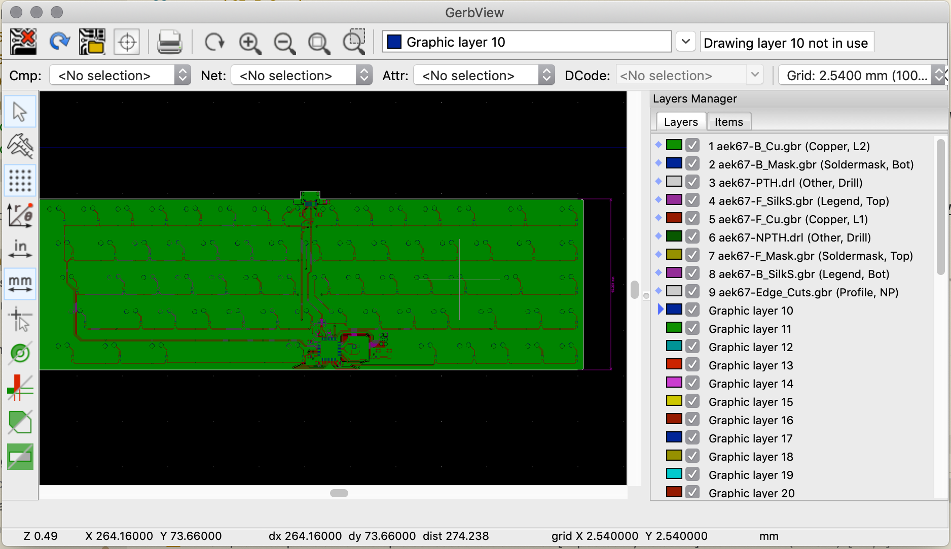
So, what to check in the viewer files?
Once this basic verification has been done, it’s time to upload the zip file to the manufacturer website. Once the file is uploaded, the site will display the gerber file. Make sure to check again the layers, as this time it’s the manufacturer interpretation of the files. With JLCPCB the interface looks like this:
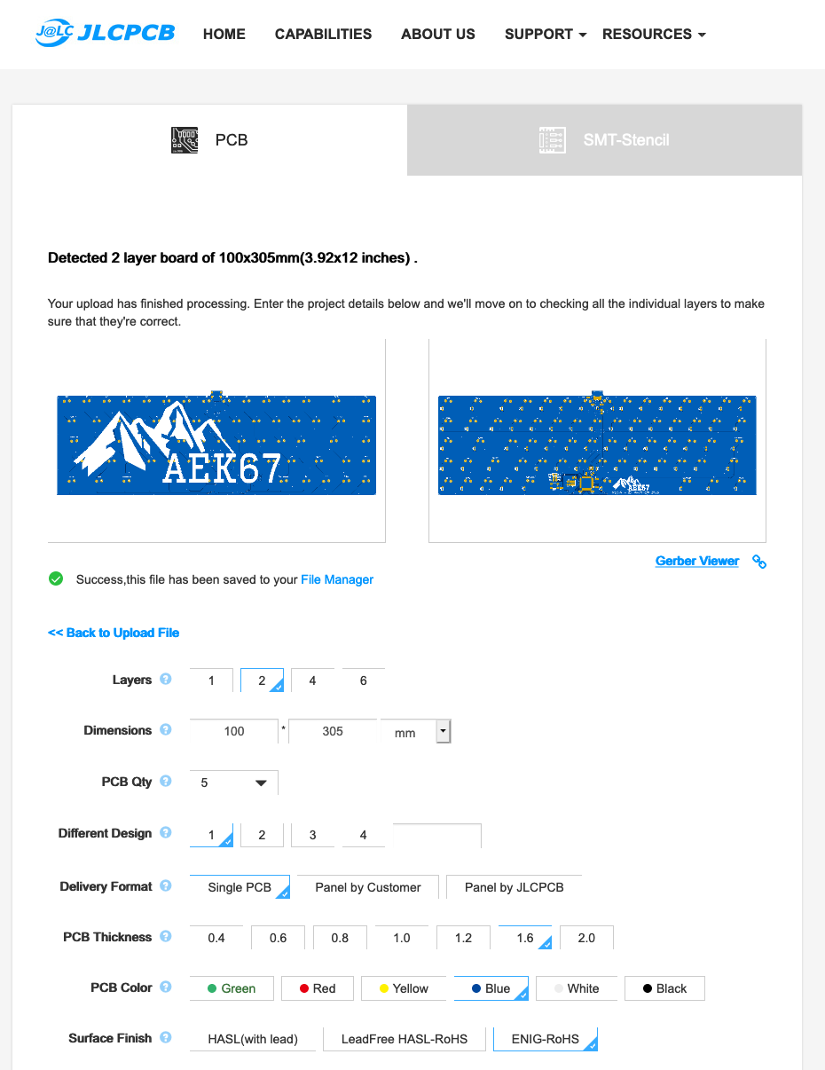
In this screenshot, I have omitted the price calculation and the bottom part (we’ll get to this one below). You can see the gerber view, and most manufacturer host an online gerber viewer to make sure the files are correctly loaded.
Immediately below, there’s the choice of number of layers and pcb dimensions. Those two numbers have been detected from the uploaded file. Make sure there’s the right number of layers (two in this case), and that the dimensions are correct. If not, check the gerber files or original Kicad files edge cutout.
The next set of options deals with the number of PCB and their panelisation:

Paneling is the process of grouping multiple PCB on the same manufacturing board. The manufacturer will group several PCB (from either the same customer or different customers) on larger PCB. You can have the option of grouping your PCB the way you want, depending on the number of different designs you uploaded. On my case, this is straightforward as there’s only one design that doesn’t need to be panelized. Even though, I’m going to build only one keyboard, the minimum order quantity is 5 pieces. But that’s not as bad as it seems, because that will leave me the freedom of failing the assembly of a few boards :)
The next set of options are the technical characteristics of the board:
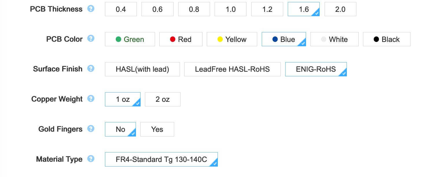
There we can change the thickness, color, finish, copper weight etc.
Those parameters are important so I need to explain what to choose. The PCB thickness represents the thickness of the FR4 fiber glass board sandwiched by the two copper layers which are later on etched to form the tracks. For a regular keyboard the standard is 1.6 mm. If you want to build a keyboard with more flex, you can opt for a 1.2 mm PCB. Note that in this case, it will not be possible to properly use PCB snap-in stabilizers (hopefully it won’t be an issue for screw-in stabilizers or plate stabilizers). Since this PCB is to be used in a regular keyboard, the default 1.6 mm is to be used.
The PCB color is a matter of preference of course. Just know that the final price is dependent on the chosen color. Most PCBs manufactured by JLCPCB are green, so this color is a lot cheaper (and take less lead/build time) than blue ones. Since the beginning of this series I was showing a blue soldermask so I decided to keep using a blue soldermask. I got a warning that it would mean two extra days of lead time.
Surface finish is how the pads and through-holes are plated. There are three possibilities, HASL, lead-free HASL, and ENIG. Technically the two first ones are equivalent.
The pads’ copper will oxidize with time at the contact with air. Those solderable parts of the PCB must be protected by a surface treatment to prevent oxidation. The HASL (Hot Air Solder Leveling) and its lead-free variant consist in dropping a small amount of solder tin-alloy on all the visible copper parts. ENIG or Electroless Nickel Immersion Gold is a plating process consisting in plating the copper with a nickel alloy and then adding a very thin layer of gold on top of it (both operations are chemical operations where the board is dipped in special solutions). I did test both options, and I really favor ENIG over HASL (despite the price increase). I found that it is easier to solder SMD components on ENIG boards than on HASL ones (the solder seems to better wet and flow, also the surface is completely flat on ENIG boards so it’s easier to place components).
The copper weight is in fact a measure of the copper thickness on each layer. The default is 1 oz, which means a thickness of 35 µm. Using a thicker copper layer would change the trace thickness and thus their electrical characteristics (inductance, impedance and such). The default of 1 oz is fine for most use cases.
Next gold fingers. This isn’t needed for most PCB (especially keyboards). Gold fingers are visible connection traces on the edge of the PCB that are used to slot-in a daughter card in a connector.
Finally for 2-layers boards, JLCPCB doesn’t offer to choose a different board material than regular FR4.
The next set of options are less important and some are straightforward:
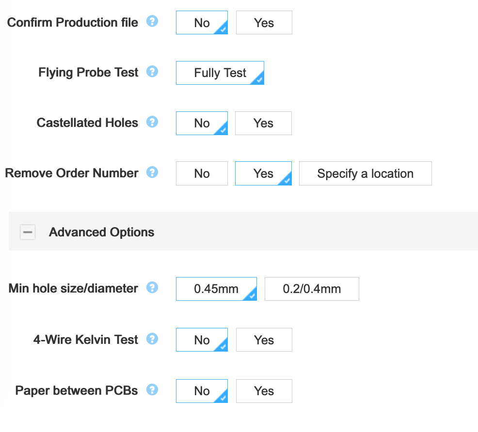
I will just talk about castellation holes. Those are plated holes at the edge of the board. They will be cut in half in the process (if the option is selected). One of the use case is to join and solder two distinct pcb by the edge, using either solder joints or specialized connectors. This option is not needed for this project.
And finally the last option is the possibility to have the pcb separated by a piece of paper when packed. JLCPCB quality is reasonably good, but I had a few of my PCBs with partly scratched silkscreen or soldermask. It’s up to you to select or not this option (it increases the price because of the extra labor).
Before ordering, it is also possible to purchase assembly. In this case, all the components will be soldered at the factory (though they only support one face and only some specific parts, USB receptacles for instance are not available). If selected, you’ll need to provide the BOM and the parts position/orientation (Kicad can gnerate this placement file, but there are some recent Kicad versions generating files with bad parts orientations). Since this would spoil the fun of soldering SMD parts by hand, I won’t select it.
It’s also possible to order a stencil. A stencil is a metal sheet with apertures at the pads locations (imagine the soldermask but as a metal sheet), here’s an example:

When soldering with a reflow oven or an hot air gun (or even an electric cooking hot plate)), the stencil is used to apply solder paste on the pads. This technique is demonstrated in this video. I don’t need this option either, as I intend to hand solder with a soldering iron the SMD components.
The next step is to finalize the order, pay and wait. Depending on the options (mostly the soldermask color), it can take from a couple of days to more than a week for the PCBs to be manufactured. Shipping to EU takes between one or two weeks depending on the chosen carrier (and the pandemic status).
A PCB without any components is of no use. So while waiting for the boards to be manufactured and shipped to me, let’s order the components.
Kicad is able to generate a BOM list with the File → Fabrication Output → BOM File... This produces a CSV file. Note that it’s not a regular CSV where fields are separated by commas, instead they are using semicolon separators. This file can be loaded into a spreadsheet software. After cleaning it a bit (removing the switches and logos), it gives this kind of table:
This will be of great help to know how many components I have to order to build one PCB (or the 5 ordered in the previous chapter).
So in a nutshell, for this keyboard, the following parts need to be sourced:
| Designation | Type | Footprint | Quantity |
|---|---|---|---|
| FB1 | Ferrite Bead | 0805 | 1 |
| SW1 | Reset switch | SKQG | 1 |
| C1-C4 | 100nF Capacitor | 0805 | 4 |
| C5 | 10uF Capacitor | 0805 | 1 |
| C6 | 1uF Capacitor | 0805 | 1 |
| C7, C8 | 22pF Capacitor | 0805 | 2 |
| R1, R2 | 10kΩ Resistor | 0805 | 2 |
| R3, R4 | 22Ω Resistor | 0805 | 2 |
| R5, R6 | 5.1kΩ Resistor | 0805 | 2 |
| X1 | 16 MHz Crystal | 3225 | 1 |
| USB1 | USB Connector | HRO-TYPE-C-31-M-12 | 1 |
| U2 | PRTR5V0U2X | SOT143B | 1 |
| U1 | Atmega 32U4-AU | TQFP-44 | 1 |
| F1 | PTC Fuse | 1206 | 1 |
| D1-D67 | Diode | SOD-123 | 67 |
First, let’s see where electronic parts can be bought. There are lots of possibilities. I don’t recommend sourcing from random stores on AliExpress, but instead ordering from professional vendors. You’ll be sure to get genuine parts (and not counterfeited components). Professional vendors will also store and ship correctly components in term of humidity and ESD protections.
I usually buy parts from the following vendors (because I’m based in the EU, I tend to favor European vendors):
I usually order from LCSC, TME and RS. With a predilection for TME lately. Almost all those vendors carry the same kind of components, sometimes even from the same manufacturers (for the most known ones like Murata, Vishay, etc). On LCSC, you’ll also find components made by smaller Chinese companies that can’t be found anywhere else.
All those vendors also provide components’ datasheets which is very useful to select the right part. For all components, I’ve added a table with links to the parts on LCSC, TME and Digikey.
The diodes are the simplest component to select. A keyboard needs basic signal switching diodes, the most iconic one is the 1N4148. I selected the SOD-123 package reference 1N4148W-TP from MCC.
| Reference | LCSC | TME | Digikey |
|---|---|---|---|
| D1-D67 | C77978 | 1N4148W-TP | 1N4148WTPMSCT-ND |
To select a PTC resettable fuse, one need to know its basic characteristics. USB is able to deliver at max 500 mA (because that’s what the 5.1 kΩ pull up resistors R5 and R6 says to the host), so ideally the fuse should trip for any current drawn above 500 mA. Based on this, I can select a part that has the 1206 SMD form factor and a reasonable voltage.
I selected the TECHFUSE nSMD025-24V on the LCSC site. It trips at 500mA, is resettable (ie once it triggers, it will stop conducting, but will become conducting again after the surge), and it can sustain up to 100A (which is large enough to absorb any electrical surge). This specific part is not available from the other vendors, but can be substituted by the Bell Fuse 0ZCJ0025AF2E (other manufacturer’s part can also match).
This component looks like this:

To summarize:
| Reference | LCSC | TME | Digikey |
|---|---|---|---|
| F1 | C70069 | 0ZCJ0025AF2E | 507-1799-1-ND |
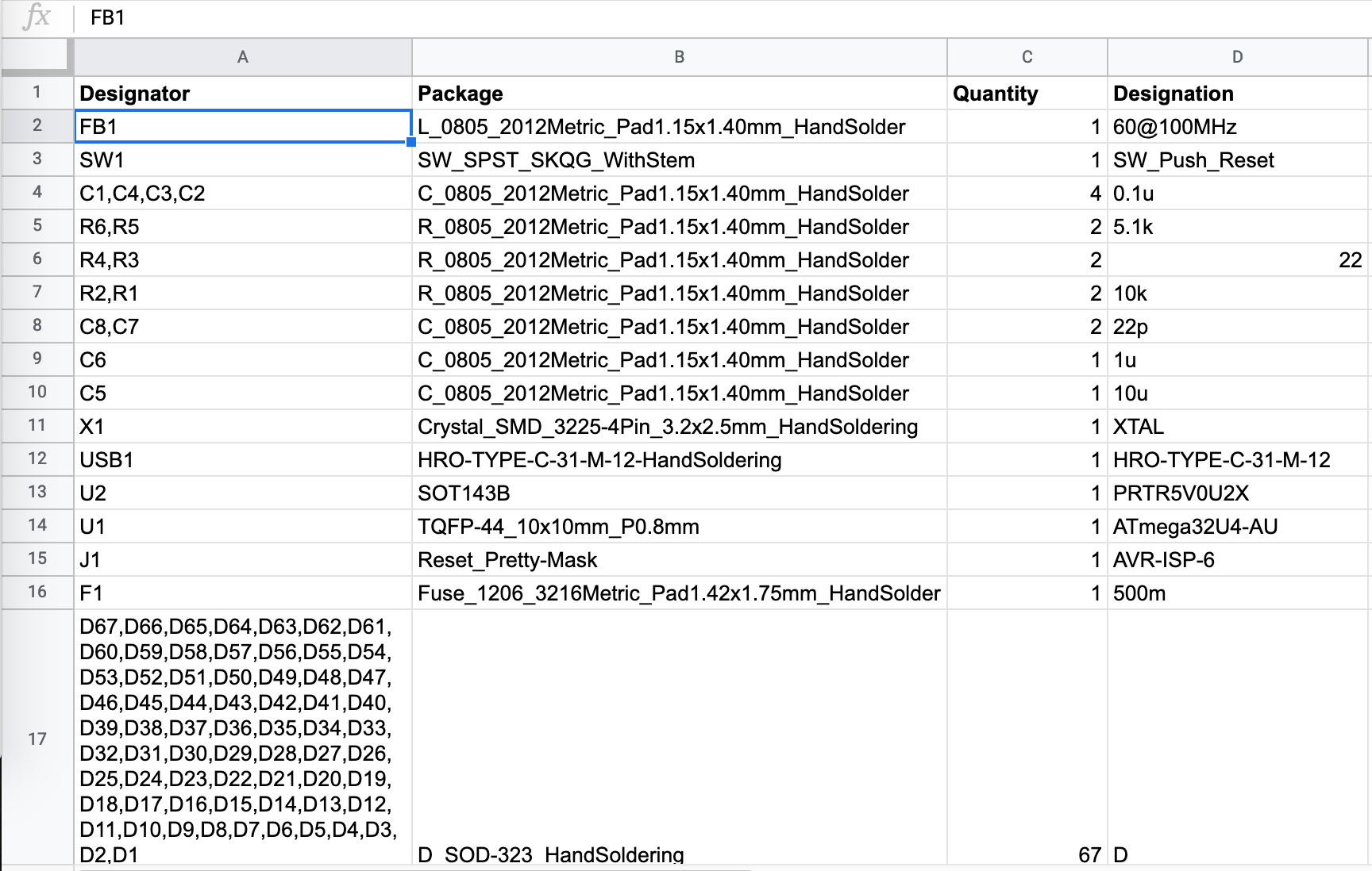
The MCU I used by default is programmed to work with a crystal oscillator (or a ceramic resonator). To select such component, the main characteristics are it’s oscillation frequency (16 MHz here) and part size (3225). In LCSC, those parts are called Crystals Resonators, but in fact they are oscillators.
The next parameter is the frequency deviation in ppm. The lower is the better. Parts with the lowest ESR should also be favored.
In a previous design, I had selected the Partron CXC3X160000GHVRN00 but LCSC now lists this part as to not be used for new designs (I have no idea why, maybe this is an EOL product). So instead it can be replaced by either the Seiko Epson X1E000021061300, the IQD LFXTAL082071 or the Abracon LLC ABM8-16.000MHZ-B2-T, or the SR PASSIVEs 3225-16m-sr.
Here’s how a crystal oscillator looks like:
| Reference | LCSC | TME | Digikey |
|---|---|---|---|
| 16 Mhz Crystal | C255909 | 3225-16m-sr | 1923-LFXTAL082071ReelCT-ND |
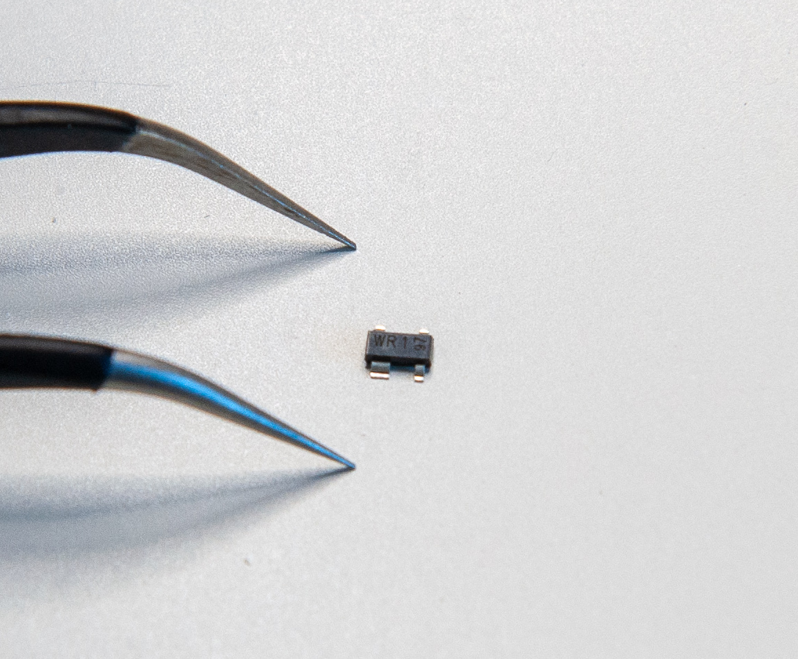
To choose resistors, the following characteristics matter:
The tolerance is the amount of variation in resistance during manufacturing from one sample to another. The lower the tolerance is, the better the resistor has the indicated value, but the higher the price is.
For most of the applications, a 10% or 5% tolerance doesn’t matter, but for some applications you might want to go down to lower tolerance values like 1% or even 0.1%. I’ve selected 1% tolerance parts, but I believe it is possible to use 5% ones.
The power is the amount of power the resistor is capable to handle without blowing. For this keyboard, 125 mW (or 1/8 W) is more than enough.
A SMD 0805 resistor (here it’s 22Ω) looks like that (yes that’s the small thing in the caliper):

Here’s a list of the selected part
| Reference | resistance | LCSC | TME | Digikey |
|---|---|---|---|---|
| R1, R2 | 10kΩ | C84376 | RC0805FR-0710KL | 311-10.0KCRCT-ND |
| R3, R4 | 22Ω | C150390 | CRCW080522R0FKEA | 541-22.0CCT-ND |
| R5, R6 | 5.1kΩ | C84375 | RC0805FR-075K1L | 311-5.10KCRCT-ND |
Note that some of those parts are available only in batch of more than 100 pieces. It is perfectly possible to substitute with parts that are sold in lower quantities as long as the characteristics are somewhat equivalent.
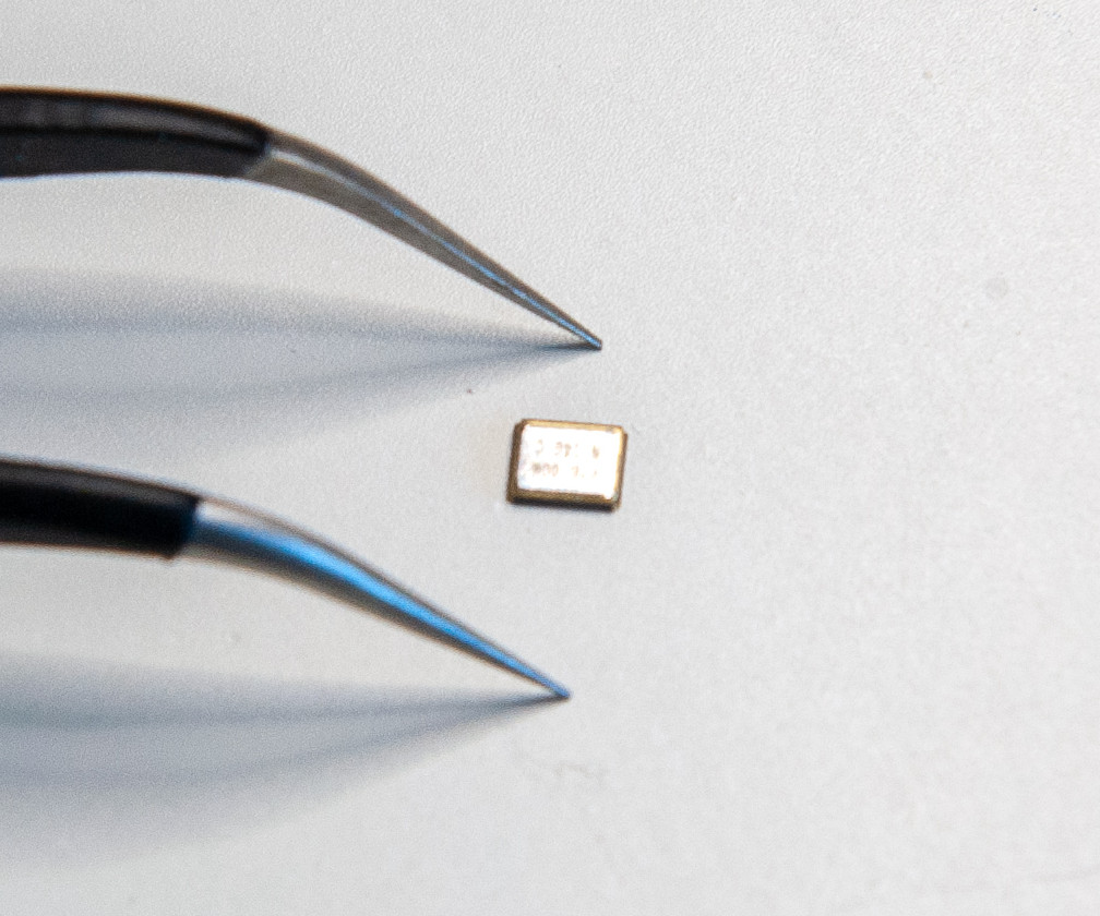
There are many type of capacitors of various conception and technology. For our decoupling/bypass SMD capacitors, MLCC (multi layered ceramic capacitors) are the best.
Here are the characteristics used to describe capacitors:
For decoupling and crystal load capacitors, it is not required to use a very precise capacitance, thus we can use the 10% tolerance. As far as this board is concerned, max voltage can be anywhere above 16V.
The temperature coefficient is (like for resistance) the variation in capacitance when temperature increases or decreases. For capacitors, it is represented as a three character code, like X7R, X5R, where:
X is -55ºC for instance)5 is 85ºC, 7 is 127ºC for instance)R means +/- 15%, but V is about +-85% (ouch).You might also find C0G (or NP0) capacitors. Those are completely different beasts (in fact it’s a complete different capacitor class), they are not affected by temperature at all.
It’s better to choose R over V variants (ie X7R is better than Y5V for instance). Since our keyboard temperature is not expected to increase considerably, X7R or even X5R can be selected. C0G parts are usually larger and harder to find in package smaller than 1206.
Among manufacturers, you can’t go wrong with AVX, Samsung, Vishay, Murata and a few others. I’ve selected Samsung parts in the table below.
Here’s how a SMD 0805 capacitor looks like:
| Reference | capacitance | LCSC | TME | Digikey | Note |
|---|---|---|---|---|---|
| C1-C4 | 100 nF | C62912 | CL21B104KBCNNNC | 1276-1003-1-ND | |
| C5 | 10 uF | C95841 | CL21A106KOQNNNG | 1276-2872-1-ND | TME only have the X5R version |
| C6 | 1 uF | C116352 | CL21B105KAFNNNE | 1276-1066-1-ND | |
| C7, C8 | 22 pF | C1804 | CL21C220JBANNNC | 1276-1047-1-ND | lower capacitance are only available in C0G |
Choosing the right ferrite bead is a bit complex. One has to dig in the various reference datasheets. This PCB needs a ferrite bead that can filter high frequencies on a large spectrum (to prevent noise coupling in GND and ESD pulses). Ferrite beads characteristics are usually given as characteristic impedance at 100 MHz. That doesn’t give any clue about the characteristic impedance at over frequencies. For that, one need to look at the frequency diagrams in the datasheet.
What I know is that, the impedance at 100 MHz should be between 50Ω and 100Ω to be effective to filter out noise and ESD pulses. For the same reason, it also needs to resist to high incoming current.
After looking at hundreds of references, I finally opted for the Murata BLM21PG600SN1D .
Also, since I opted for a 0805 package, its current limit is in the lower part of the scale. I might probably change the PCB in an ucoming revision to use a 1206 sized ferrite bead to have it support higher currents.
| Reference | LCSC | TME | Digikey |
|---|---|---|---|
| FB1 | C18305 | BLM21PG600SN1D | 490-1053-1-ND |
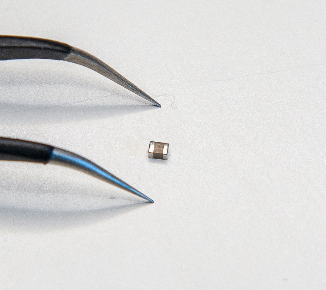
| Reference | LCSC | TME | Digikey | Note |
|---|---|---|---|---|
| PRTR5V0U2X | C12333 | PRTR5V0U2X.215 | 1727-3884-1-ND | |
| AtMega32U4-AU | C44854 | AtMega32U4-AU | ATMEGA32U4-AU-ND | |
| HRO-TYPE-C-31-M-12 | C165948 | not found | not found | |
| Reset Switch | C221929 | SKQGABE010 | CKN10361CT-ND | TME doesn’t carry the C&K switch, so substituted by the Alps version |
Here’s a picture of the PRTR5V0U2X, notice the GND pin that is larger than the other ones:
SMD components are packaged in tape reels. If you purchase less than a full reel (4000 to 5000 individual pieces), you’ll get a cut piece of the tape like this one:
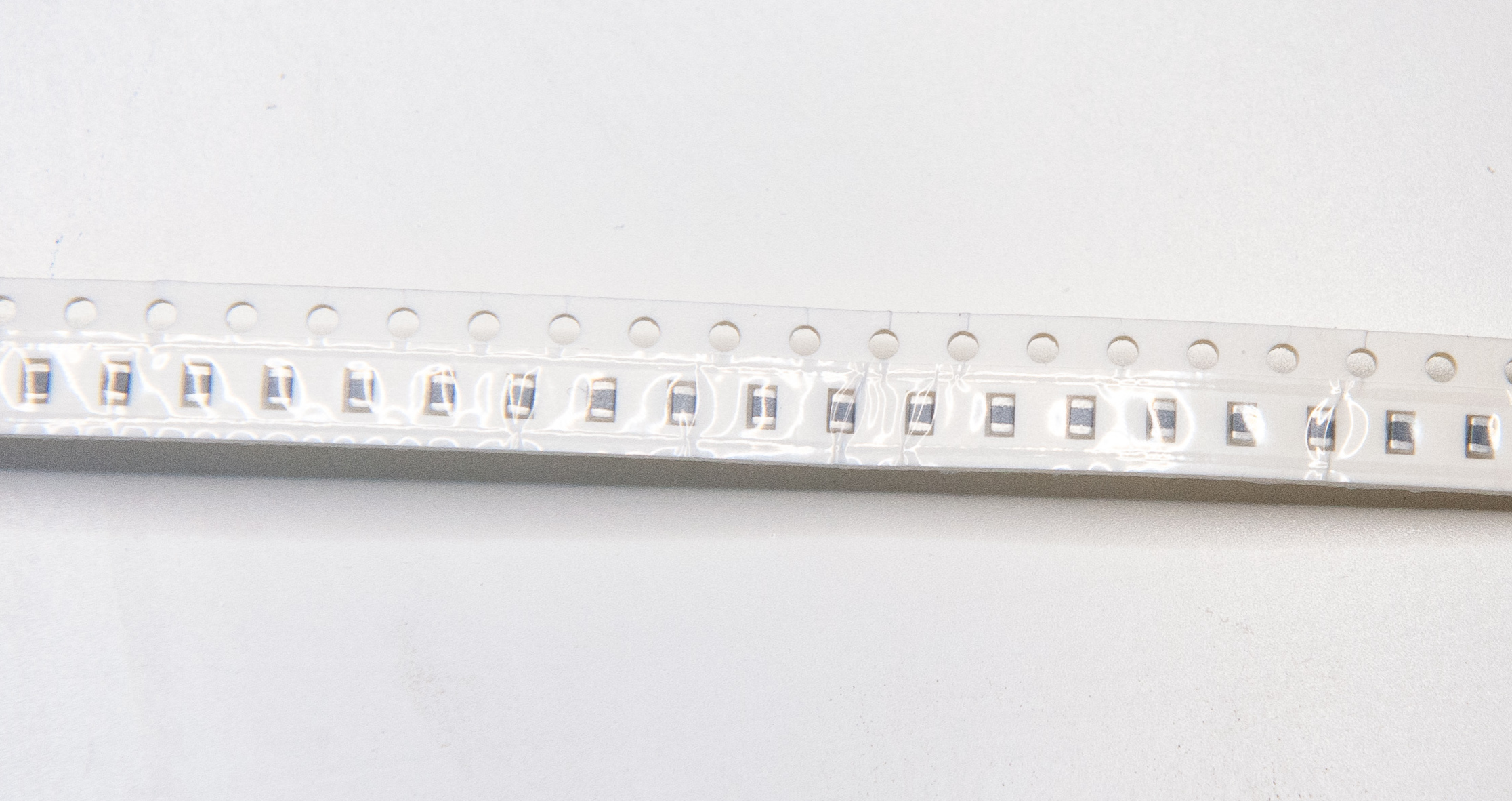
Those tapes are made of two parts: a small shiny transparent layer on the top (the cover tape) and the bottom the carrier tape. To get access to the component, you just need to peel off the top layer. Since those parts are very small, I recommend to keep them in their tape and peel off only the needed portion of the cover tape.
Components are sensible to electrostatic discharge (ESD), that’s why they’re shipped in special anti-static bags. There are two types of anti-static bags. The first kind is dissipative antistatic bags, usually made from polyethylene with a static dissipative coating. They work by dissipating the static charge that could build up on their surface onto other objects (including air) when the bag is touching something else. Those are usually red or pink:

The second kind is conductive antistatic bags, made with a conductive metal layer on top of a dielectric layer. Those bags protect their contents from ESD, because the metal layer forms a Faraday cage. You can recognize those bags because they are shiny and their color is gray or silver:
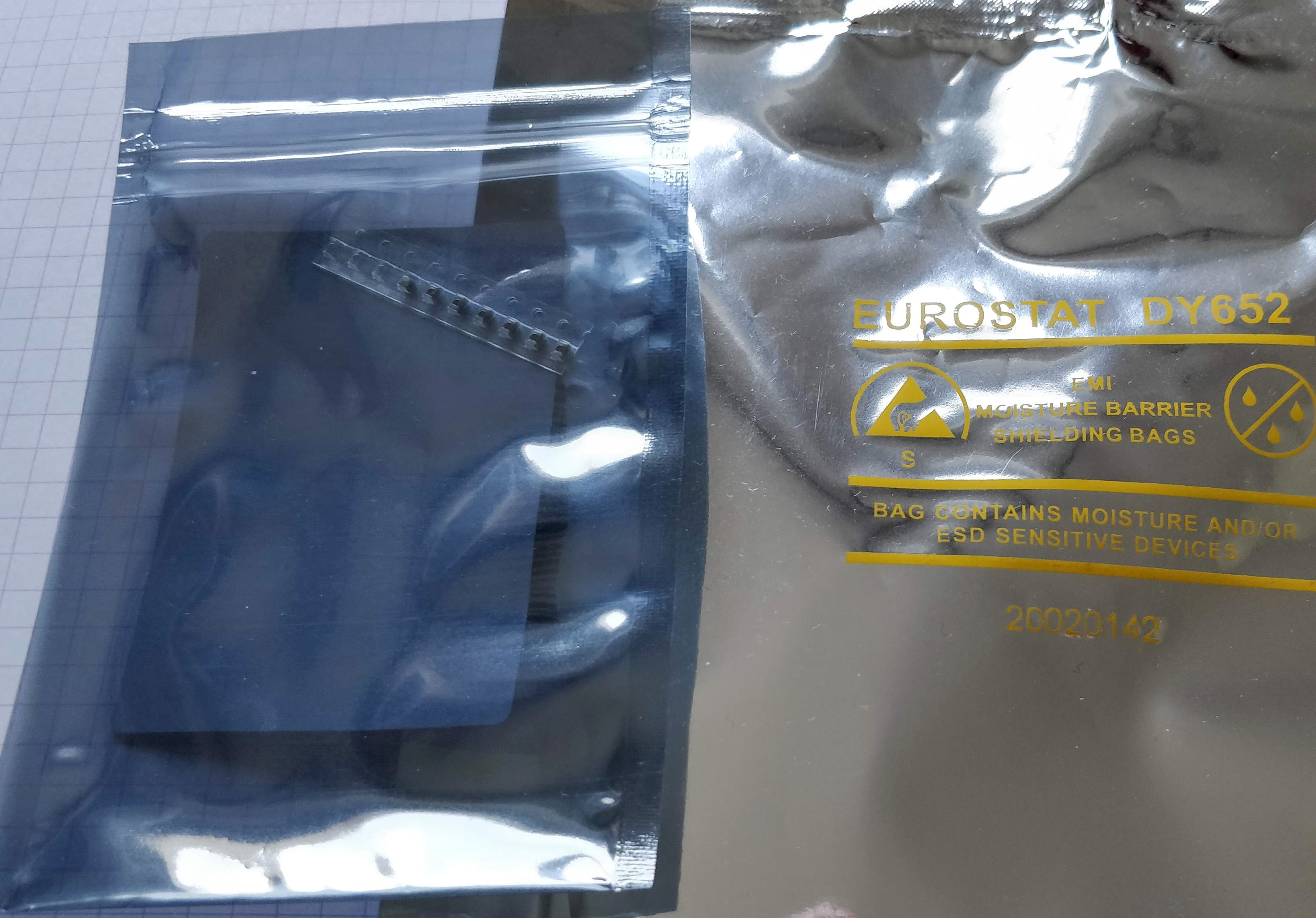
Note that those shielded bags are inefficient if the shield is not continuous, so make sure to not use bags with a perforation or puncture.
Components should always be stored in such bags, even for storage. Only remove the components from the bag when you’re ready to solder them on a PCB. And do so if possible in an anti-static environment (ie a specific table or mat is used).
Components should also be stored in a place that is not too humid. Some active components are shipped with desiccant bags inside the ESD protection bag, keep them when storing them as they absorb the excess humidity that could harm the part.
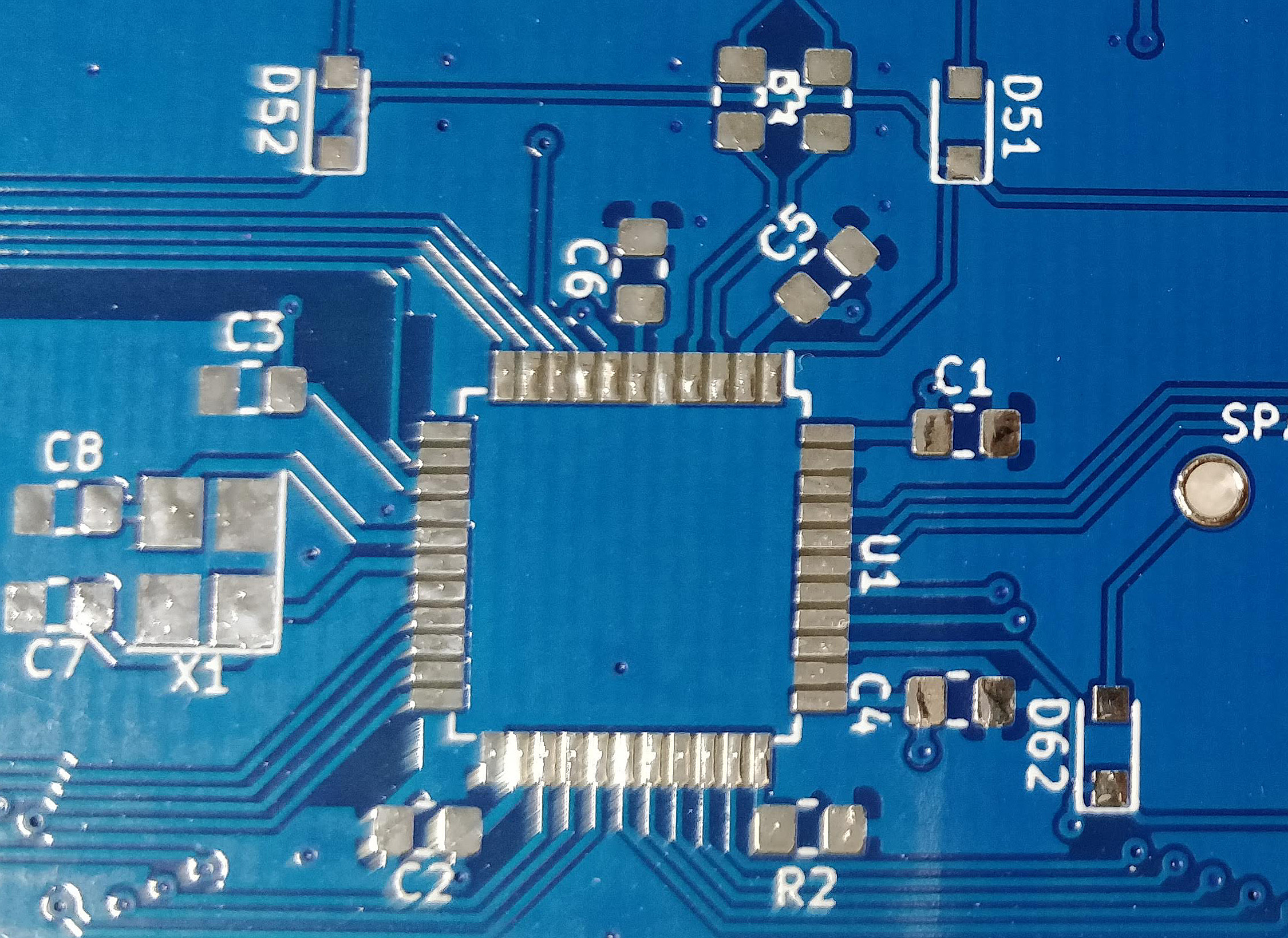
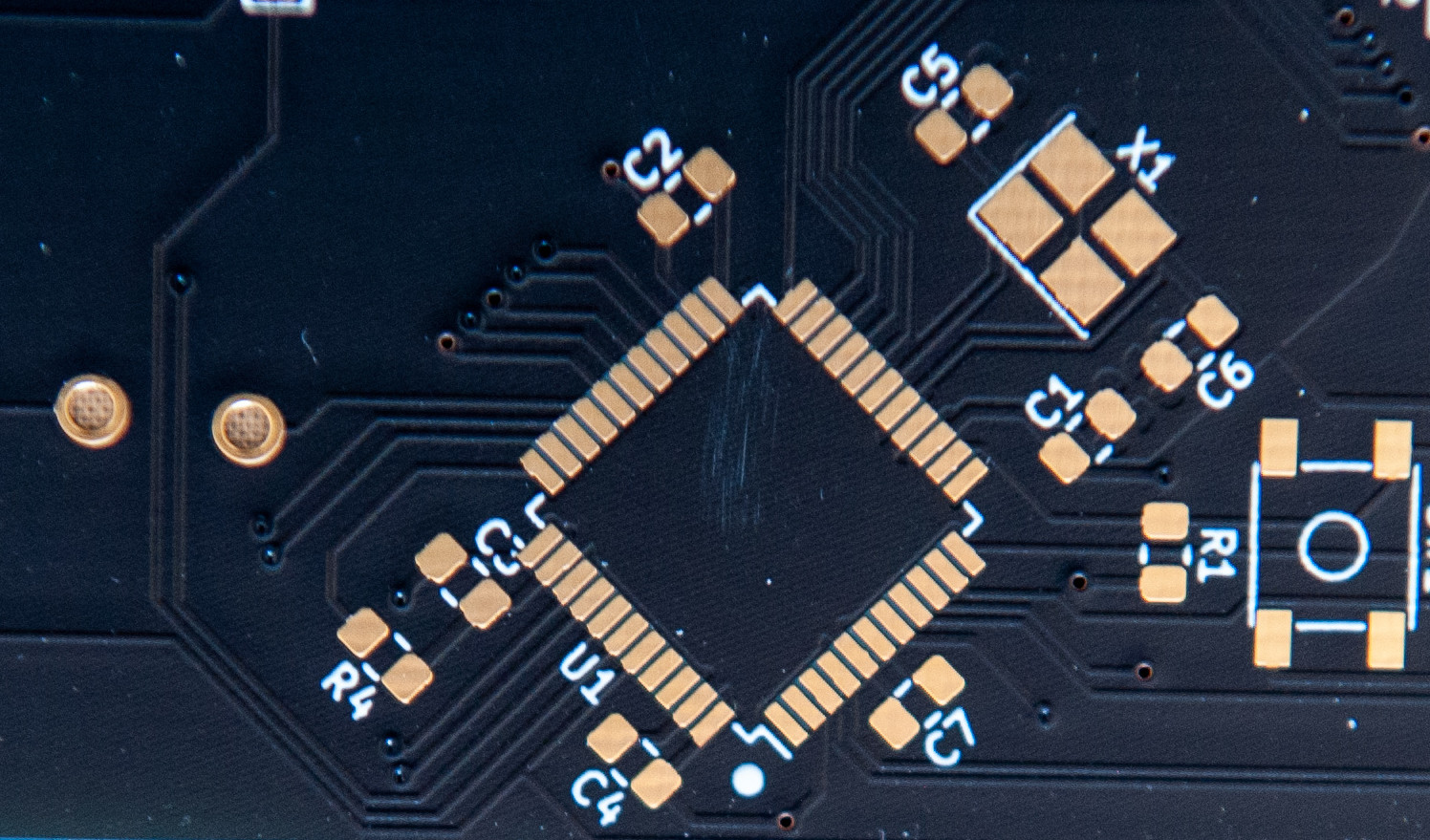
So, it’s mail day: I received the PCB:


and the components (see the AtMega32U4 in the cardboard box in the center):
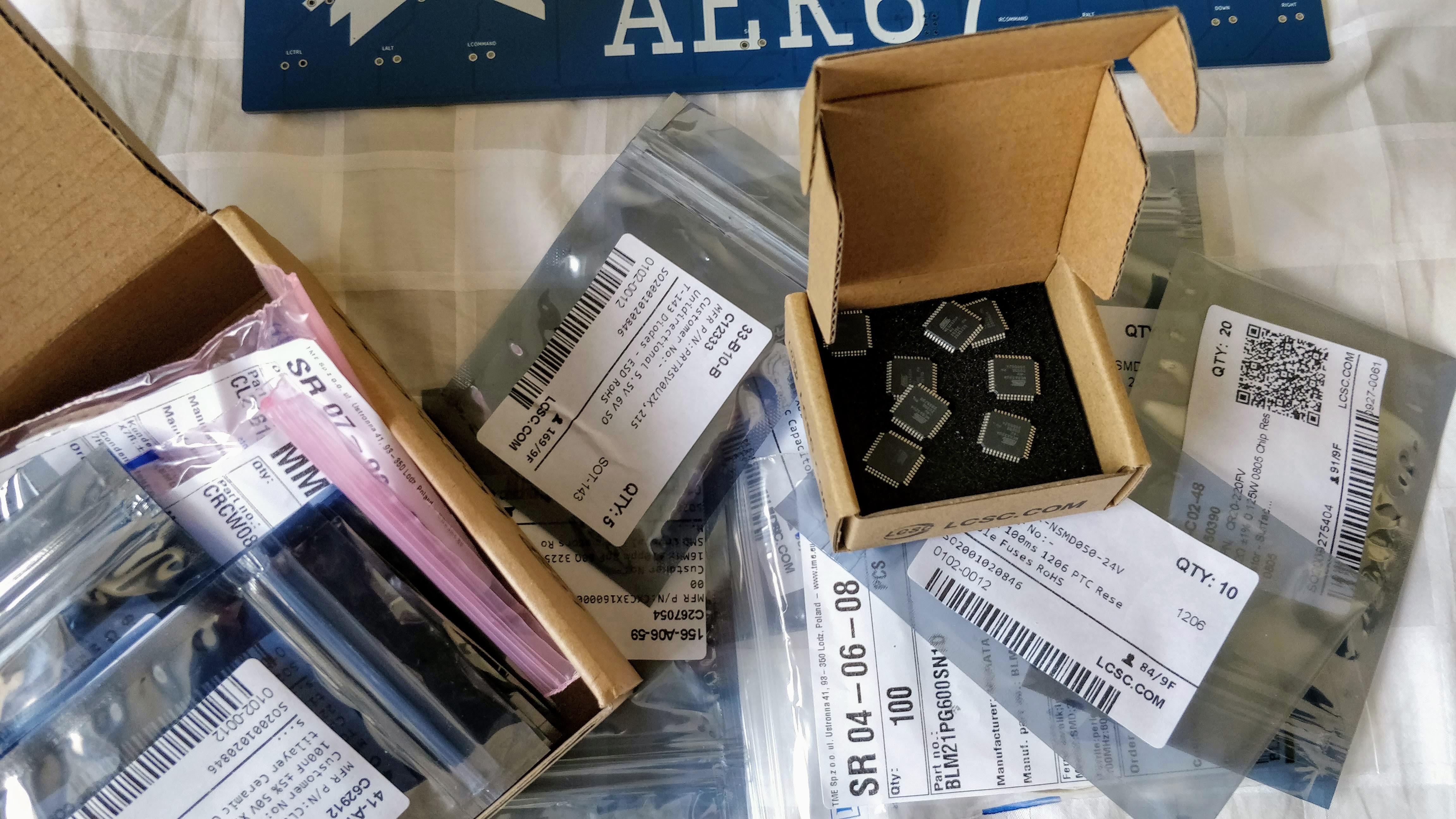
I’m now ready to assemble the PCB, that is solder all the components.
To do that the following tools are needed:
That’s the minimum required. Of course if you can afford a microscope or a binocular that would be awesome (I don’t have one, so that’s not strictly needed)
As I’ve explained earlier, electronic components can be destroyed by electro-static discharges. The human body is able to accumulate charges (for instance on walking on a carpet) and when touching another object discharge into it. Thus it’s important to prevent ESD when manipulating components.
To be able to place precisely the component on the PCB while soldering it, and also hold it while the solder solidifies, we need a pair of electronic tweezers. Since usually tweezers are made of metal, they would conduct the static charge to the component or the board. ESD tweezers are metallic tweezers that are coated with an non-conductive anti-static material, preventing the charges to be transferred from the body to the component.
You can find cheap tweezer sets at Amazon or more expensive ones at the previous vendors I cited for sourcing components.
Here are mine:

I’ll recommend using a temperature controlled soldering iron, especially for soldering very small parts. One good choice would be either the Hakko FX888D, the FX951 or any other serious temperature controlled stations (among those made by Weller or Metcalf for instance). Hakko stations can be purchased in EU from batterfly.
You’ll also find Hakko T12 compatible stations on Aliexpress (like the KSGER T12), those are nice and inexpensive, unfortunately their PSU is rigged with defective designs that make them not as secure as they should (they probably wouldn’t pass CE conformity as is). I thus won’t recommend them (see this video for more information).
Then finally you can find standalone USB powered soldering irons like the TS80P or TS100. Those are very lightweight and have a custom opensource firmware superior to the original. They have a drawback: they’re not earthed by default and thus not completely ESD safe. The risk is a potential ESD destroying the SMD components that are being soldered. Regular wall-in soldering irons have the heating tip earthed and thus can’t build up an electrostatic charge. Moreover, those USB soldering iron are known to leak current when used. This can be fixed by adding an earth connection from the iron to common earth which requires a specific cable from the iron to an earth point (or at least a common potential point between you, the iron and the PCB, which can be done with specific anti-static workbench or mats). Some TS80P kits contain such earth grounding cables, some other not. I’m reluctant to recommand those for these reasons.
I myself have an inexpensive Velleman station (made in China). It’s certainly not the best, but it does its job reasonably well and is CE certified.
Rergarding soldering iron tips, you can find many different ones and it will depend on the soldering iron you’ve got. There are tons of different Hakko tips (here for the T12 tips). In this brand, the recommended ones for SMD parts are shapes D, BC/C and B. Regarding tip size, you can’t go wrong with D12 (or D16), B2 and BC2.
The soldering iron tip is critical for the tool performance. If it can’t perform its function of transferring heat to the solder joint, the soldering iron will not be efficient. Thus it is important to take care of the tip to prevent any soldering issues.
Soldering tips will wear throughout the time of use and will probably have to be replaced at some point. Careful tip hygiene will extend its life.
A particularly recommended tool is a metallic wool, like the Hakko 599b or a cheap clone:

Those cleaners are preferred other wet sponges, because the sponges will reduce the temperature of the iron tip when used, which means the tip will contract and expand quickly during cleaning. Frequent use of the sponge will cause metal fatigue and ultimately tip failure. Metallic wool cleaners are very effective at removing the dirt, contaminants, and flux or solder residues.
The idea is to prevent oxidation, for this, clean the tip before using the soldering iron on a new component, not after. While the tip is not used between two components, the flux and solder will protect the tip from oxidation.
When you’ve finished your soldering job, clean the tip with the metallic wool and tin the tip. It is possible to buy a tip tinning box. Most large solder manufacturer produce this kind of product, mine is this reference:

You might see recommandation of applying solder on the iron tip after use. This works fine if the solder contains a rosin activated flux (see below). But for no-clean solder (the majority of solder nowadays), the flux is not aggressive enough to remove or prevent tip oxidation. I recommend using a special tip tinner as the one above.
The solder is an alloy that melts from the heat of the iron to form the joint between the PCB pad and the component. It is important to purchase a good quality solder (especially if you have to perform some rework). There are two types of solder, those that contains lead and the lead-free variant. The latter is better for health and environment, but might be harder to use because it requires a higher soldering temperature. The former is easier to deal with, but is forbidden in EU because of RoHS compliance (it’s still possible to purchase leaded solder though).
Solder should also contain flux (even though as you’ll see later, adding flux is necessary to properly solder SMD components). The flux purpose is to clean the surfaces so that the solder wet correctly and adheres to the pad and components.
Solders are described by their content, like for instance Sn60Pb40, Sn63Pb37 or Sn96.5Ag3Cu0.5. It’s simply the percentage of their constituents. For instance Sn63Pb37 is an alloy made of 63% of tin and 37% of lead. Unleaded solder is mostly made of tin and silver, and sometimes a low level of copper.
For beginners, Sn63Pb37 would be the simplest solder to use. It is an eutectic alloy. This means that the alloy has a melting point lower than the melting point of any of its constituents (or any other variation mix of tin and lead), and that it has a very short solidifying phase. This makes this kind of solder easy to work with.
Unleaded solder have a higher melting point (around 220ºC) that might take time to be accustomed to.
Well, that doesn’t give you the temperature at which you’ll have to solder the components. For SMD parts, with leaded solder, I usually set my iron between 310ºC and 320ºC. This is high enough to quickly heat the pads. Lower temperature would mean to keep the iron tip longer on the pad and component with the risk of heating too much the component. Unlike common thought, the heat conductivity of metal decreases with temperature, which means that using a lower temperature would mean more heat accumulating in the component (because of the iron tip staying longer on the pad and component), and an increased risk of destroying it.
For unleaded solder, the recommended iron temperature is around 350ºC. But it also depends on the iron tip used. Smaller iron tips have a lower heat transfer surface and thus, you will need to use a larger temperature and longer soldering to achieve the same effect as with a larger tip.
Using a solder containing rosin flux is also recommended. The metallic surfaces in contact with air will oxidize, preventing the chemical reaction that will bond them to the solder during the soldering. Oxidization happens all of the time. However, it happens faster at higher temperatures (as when soldering). The flux cleans the metal surfaces and reacts with the oxide layer, leaving a surface primed for a good solder joint. The flux remains on the surface of the metal while you’re soldering, which prevents additional oxides from forming due to the high heat of the soldering process.
As with solder, there are several types of flux, each with their own key uses and limitations:
It’s still not finished about solder. How to choose the appropriate solder diameter? A good compromise for soldering a combination of SMD parts and through-hole components is 0.7 or 0.8mm.
Finally, soldering is a health hazard, so make sure to read the following important warnings:
Among the various brands of solder, those are known to produce good solder: MgChemicals, Kester, Weller, Stannol, Multicore, Felder, MBO etc. For a thorough comparison of several brands and models, you can watch SDG video: What’s the best solder for electronics
If you solder more than occasionally it might be worth investing in a small fume extractor like this Weller WSA350 or the Hakko FA-400.
The flux contained in the solder will not be enough to solder SMD parts. It is recommended to add extra flux before soldering the components, especially for ICs or fine pitch components (see below for the different techniques).
Flux exists in several forms:
Here’s a flux pen:

And a flux serynge (ready to be used):
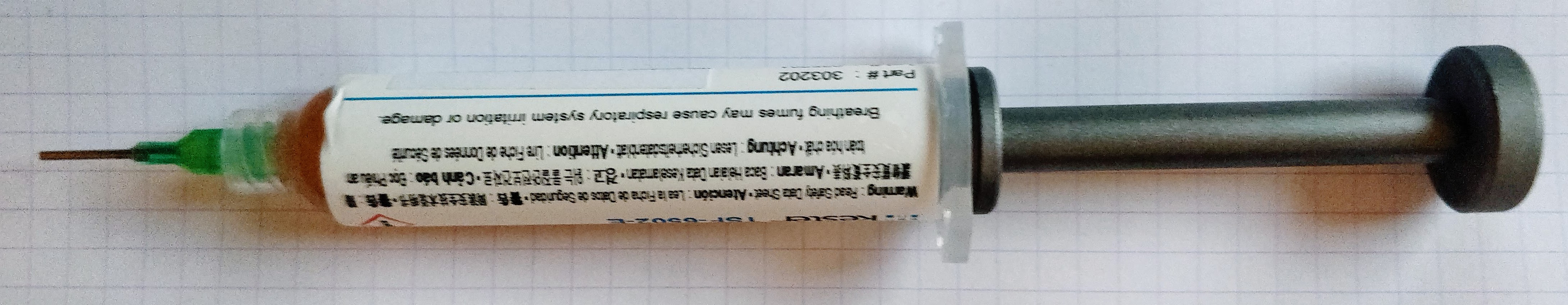
A note on flux serynge: most of them are sold without an applying nozzle and a plunger. That’s because professionals are using special dispensers. So do not forget to also purchase a plunger (they are dependent on the serynge volume) and nozzles. The nozzles are secured to the serynge by what is called a luer lock, which is a kind of threading inside the serynge.
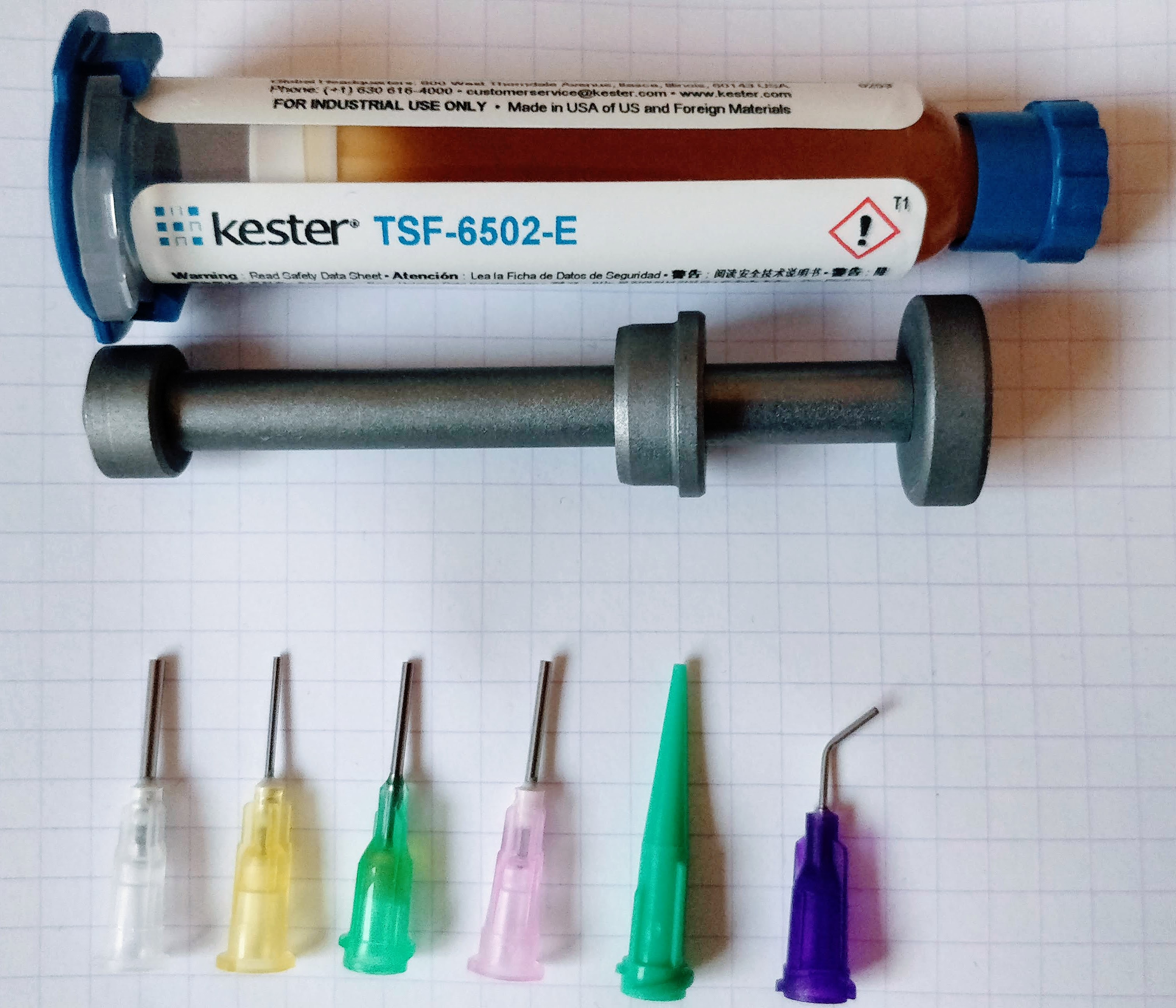
I recommend getting a flux paste serynge, as the flux from the pen is more liquid and tends to dry more quickly than the paste.
For a comparison of fluxes, you can watch the SDG video: what’s the best flux for soldering
Mistakes happens :) so better be ready to deal with them. It might be necessary to remove extra solder or remove a component misplaced by mistake. Without investing a lot of money in a desoldering iron or station, it is possible to get inexpensive tools that will help.
Let me introduce you to the desoldering pump and its friend the solder wick:

The top object in the picture is a desoldering pump. You arm it by pressing down the plunger. When released with the button, it will suck up the melted solder. It is to be used with the soldering iron heating the excess solder, then quickly apply the pump.
The solder wick is to be placed on the excess solder, then put the iron tip on top of it, the solder will melt and the wick will also suck it. It might be necessary to add a bit of flux before.
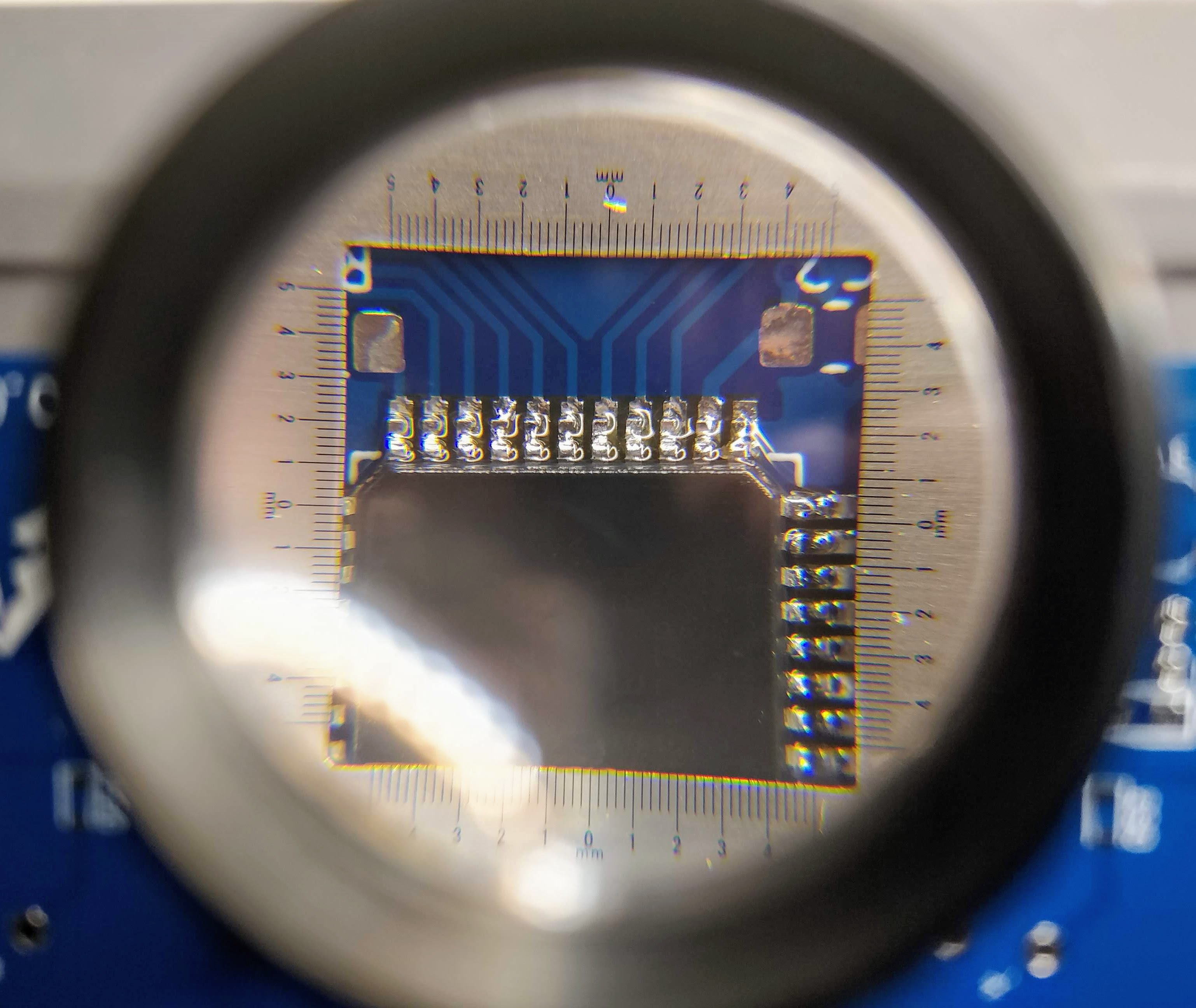
Finally the last tool needed when soldering small SMD parts is a good lamp with an integrated magnifier glass. As seen earlier, most of the component are less than 3 or 2 mm long, so it is hard to properly see them when soldering (unless you have very good eyes, which is not my case).
Of course getting a binocular or a microscope would be awesomely useful, but those are quite expensive (especially if you want quality). Instead I think a good magnifying glass lamp can do the job quite efficiently. The best ones are the Waldman Tevisio, unfortunately they are very expensive. It is possible to find cheaper alternatives on Amazon or one of the parts vendors I previously cited (I got myself this RS Online model).
The magnifying lens of such lamp is expressed in diopters. You can compute the magnifying ratio with the D/4+1 formula. A 5d lens will provide a 2.25x magnification. This is enough to solder small parts, but my experience (and bad eyes) show that when there’s a small defect its quite hard to have a good view of it (like when there’s a small bridge on two close pins on high-pitched ICs).
That’s why I also recommend getting a standalone small jewelry 10x magnifying glass. The Japanese Engineer SL-56 does an excellent work.
Enough about the tools, let’s see how to assemble the components on the PCB. First let me explain how to solder SMD parts. The technique is the same for 2 pads or multiple pads, except for fine pitch ICs which will be covered afterwards.
I’m very sorry for the bad pictures and schemas that appears in the two next sections. I unfortunately don’t have a macro lens for my camera, and my drawing skills are, well, very low :)
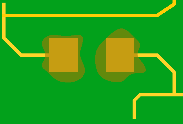
First apply a small amount of flux paste on both pads:
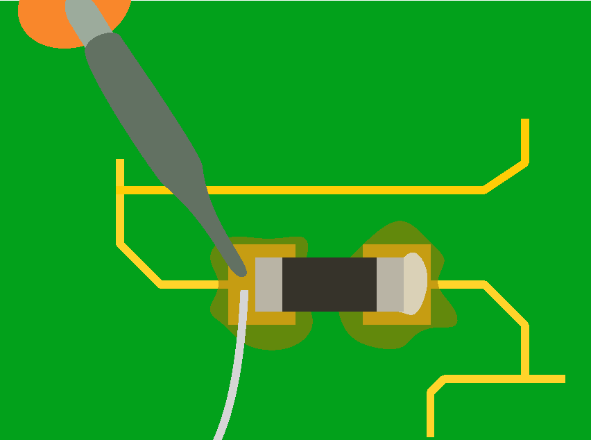
Next, wet a small amount of solder on one of the pad with the soldering iron:

Then place the component with the tweezers, hold it firmly in place and reflow the solder on the pad until the joint is formed:

Once the solder has solidified, solder the other pad normally:
On a real component (here a 5.1k resistor near the USB receptacle), this give these steps:
Adding flux:
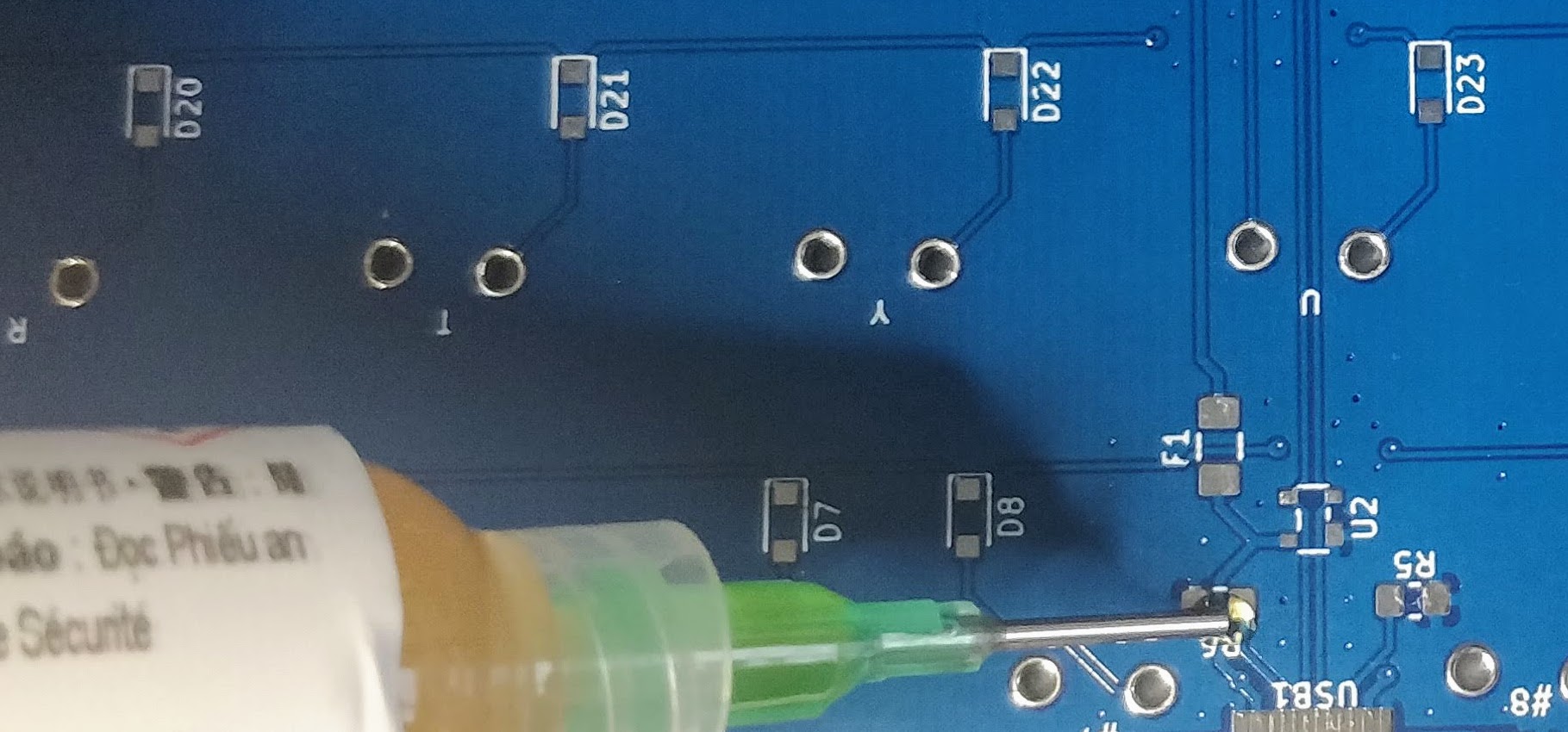
Apply some solder on one of the pad:
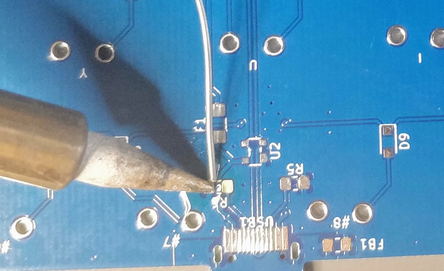
Place the component:

And since I don’t have three hands (and need one to take the picture), I soldered the first pad without holding the component (most of the time, when there’s enough flux the component will place itself correctly):
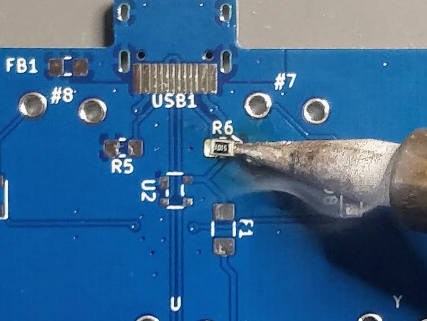
And the result (granted the component could be better aligned, the picture has been taken through the SL-56 magnifying glass):

This very same technique can also be applied to 3 or 4 legged components. Start by soldering one pin, making sure the component is correctly placed, then add solder on the other pins.
The previous soldering technique doesn’t work for fine pitch components like ICs or the USB receptacle on this PCB. For this we need a different technique: drag soldering.
The drag soldering technique consists in first soldering 2 opposite pads of an IC, then to drag the soldering iron tip and solder along the pins relatively quickly. The flux and soldermask will do their job and solder will flow only on the metal parts. Bridges can happen if there’s too much solder or the iron tip is not moved quickly enough. That’s where the solder wick is useful to remove the excess solder.
To properly drag solder, first add solder on two opposite pads of the IC. Then carefully place the IC with the tweezers, hold it firmly and reflow those two pads (this is the same technique as for 2 pins components). When the solder solidifies and form a joint, the IC is secured at the right place, and we can start drag soldering.
Here’s a small schema illustrating the technique:

You’ll find the technique shown in this drag soldering video. Notice the tip shape used in the video (equivalent to a T12 BC), and how the solder is put under the tip. If you don’t use a slanted tip, you can still put some solder on the iron, or use what I described above, moving the solder at the same time as the iron tip.
So I’m ready to solder the PCB with the aforementioned techniques. Since it’s harder to solder fine pitch components, it’s better to start with them. There’s nothing worst than soldering all 2-pads components, then failing soldering the most complex one and having to thrash the board.
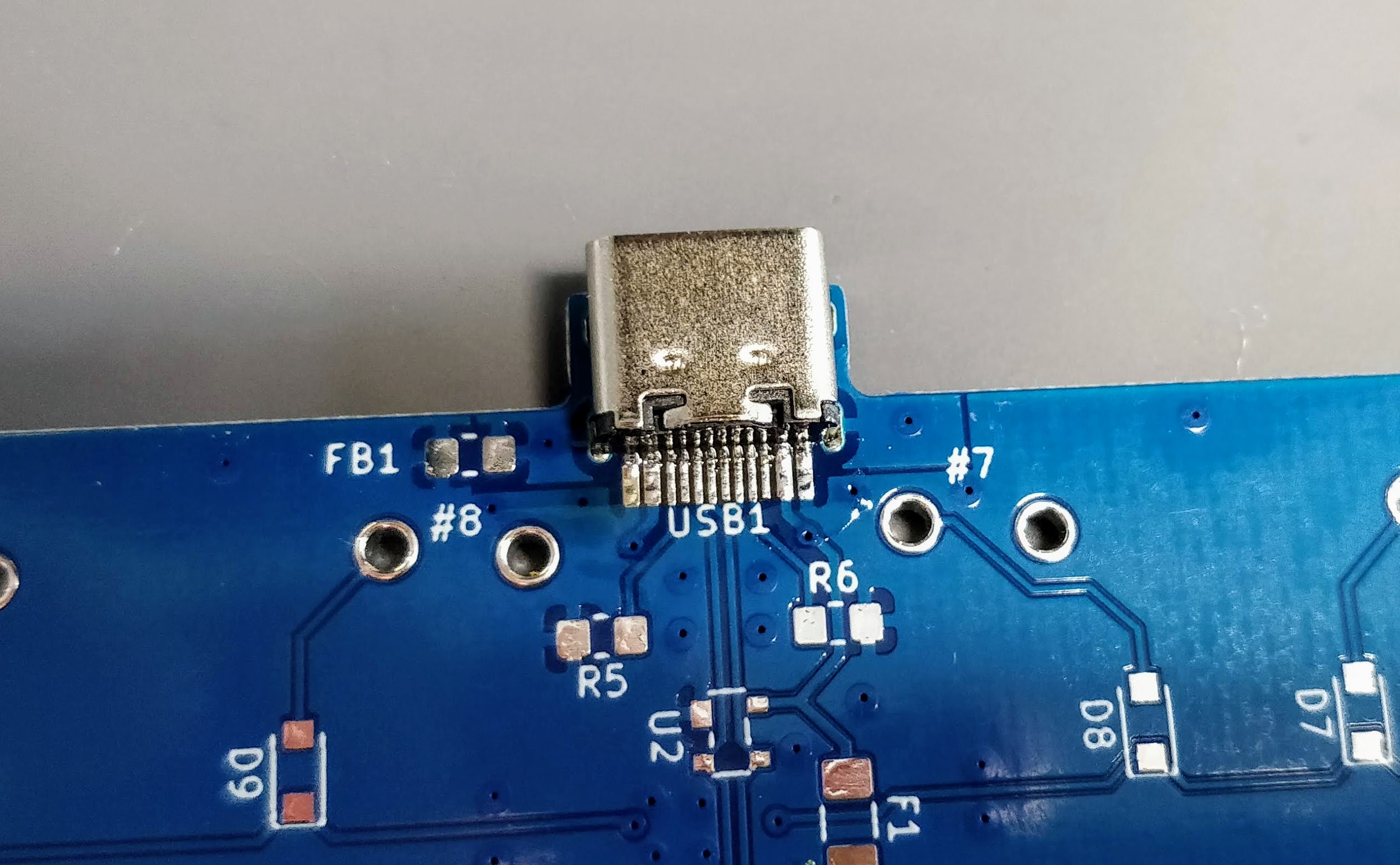
My advice is to start by soldering the USB connector first. Place it so that the small pins enter the board and solder on the front side. The USB connector is then now in place and the small pins are exactly placed on top of the pads on the back side of the PCB:
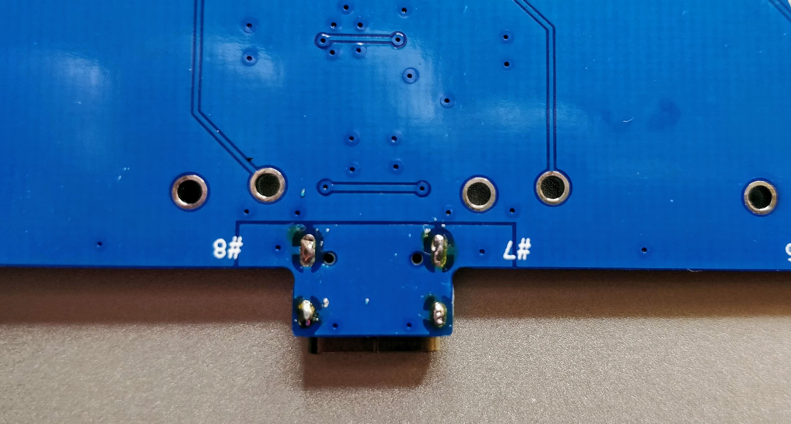
Then apply some flux paste on the other side accross the pins:
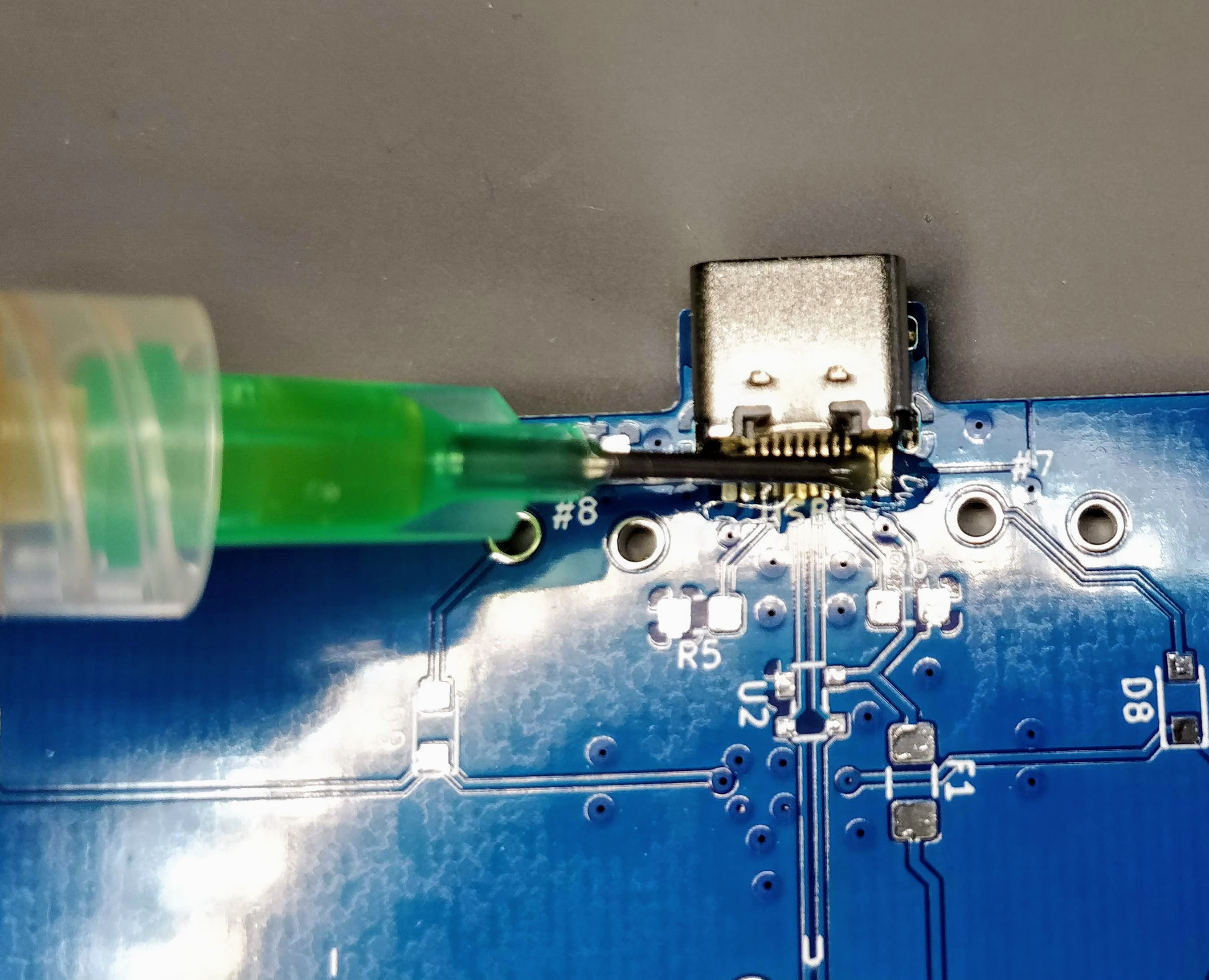
And drag solder the connector. This will give this (flux have been removed in the following picture):
Now is a good time to visually inspect there’s no bridge. Then it might also be a good idea to test that there’s no Vcc and GND short with a multimeter. Most multimeter (even the cheapest ones) have a “diode test” or continuity mode. In this mode the multimeter sends a very small current across the probes and measures the voltage. When the resistance is very small (if there’s electrical continuity between them) the multimeter will produce a beep. If there’s no continuity there won’t be any beep and the screen will show something specific (on mine it displays 1 which is very misleading).
With the multimeter in continuity testing mode, put the black probe on one of the GND pin and the other on one of the Vcc pin (or reverse, it doesn’t matter). There shouldn’t be any continuity (or beep). If there’s continuity, it means there’s a bridge that needs to be found and repaired by adding flux and using the iron tip or with the help of solder wick. You can test the other pins, there shouldn’t be any continuity except for pins that are doubled (D+/D-, GND, Vcc).
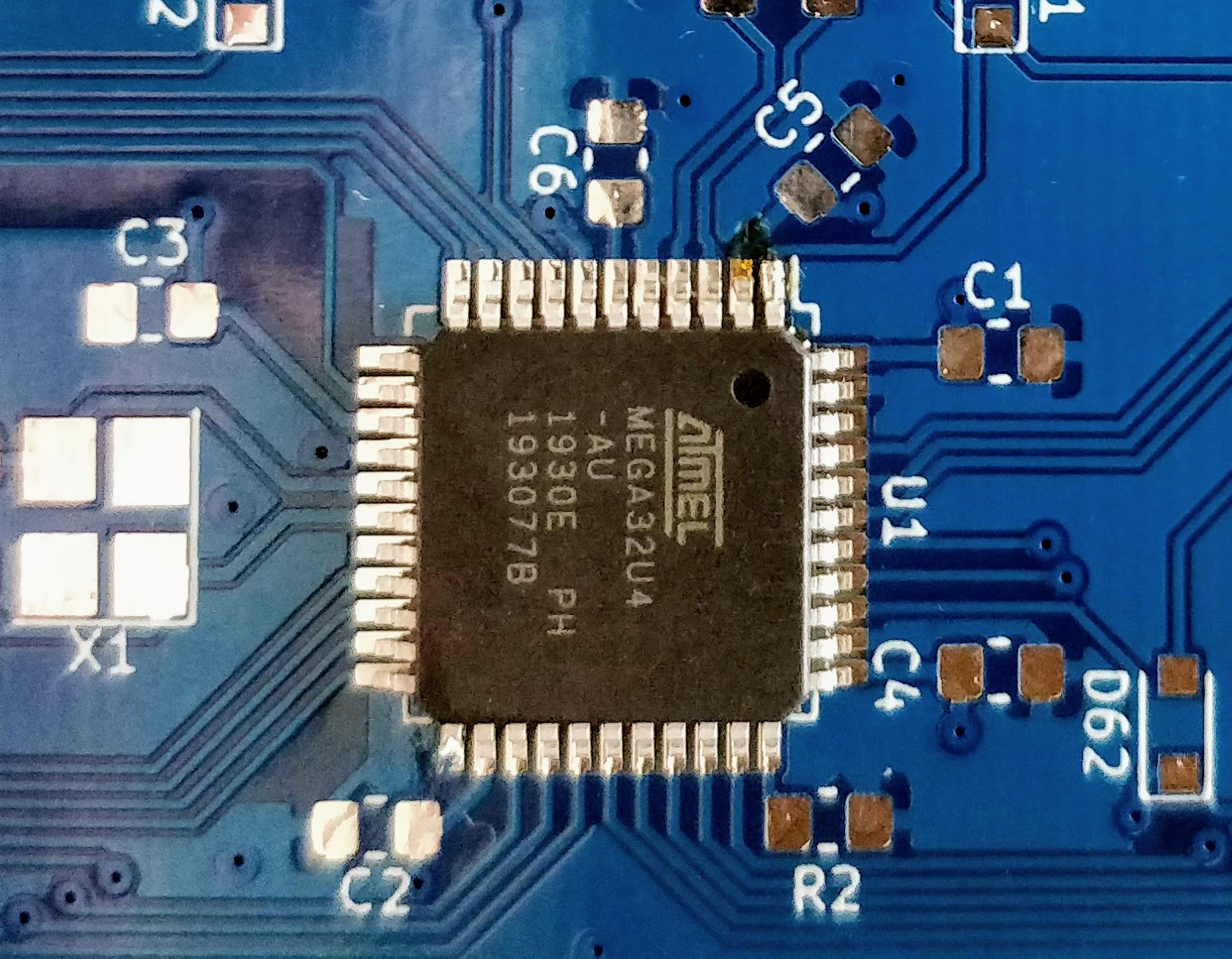
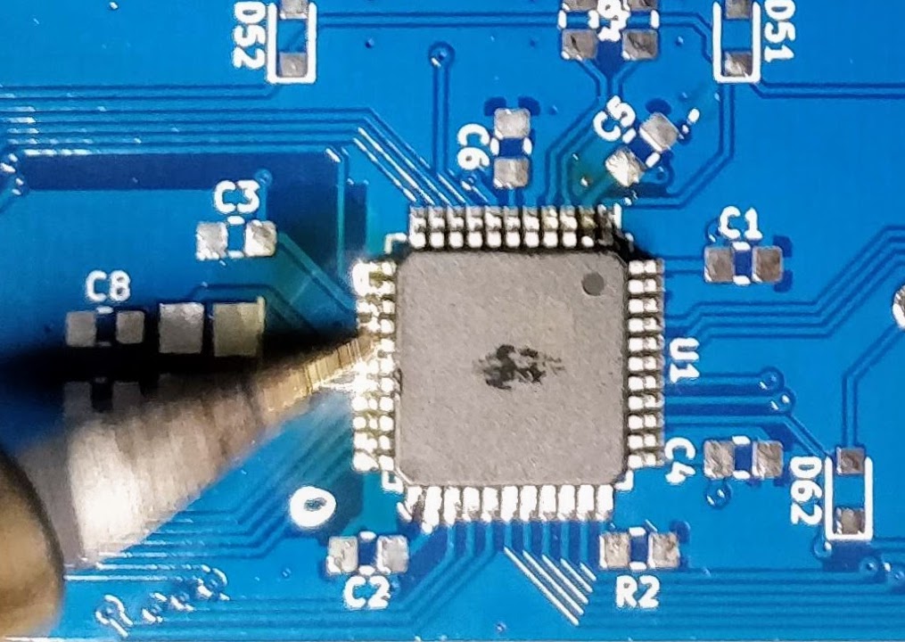
If everything is OK, the next step is to solder the AtMega32U4 MCU. First make sure to check how it should be placed. The silkscreen printed at the back of the board contains a small artifact indicating where pin 1 is. On the chip, the pin 1 is the pin close to the small point.
To make sure I’m soldering the component at the right place, I can use the Interactive HTML BOM plugin for Kicad. In the Kicad PCB editor, the plugin can be launched with Tools → External Plugins… → Generate Interactive HTML BOM. In the HTML Defaults section, it’s a good idea to select Highlight first pin and Layer View → Back only. After pressing Generate BOM, a web browser opens containing:
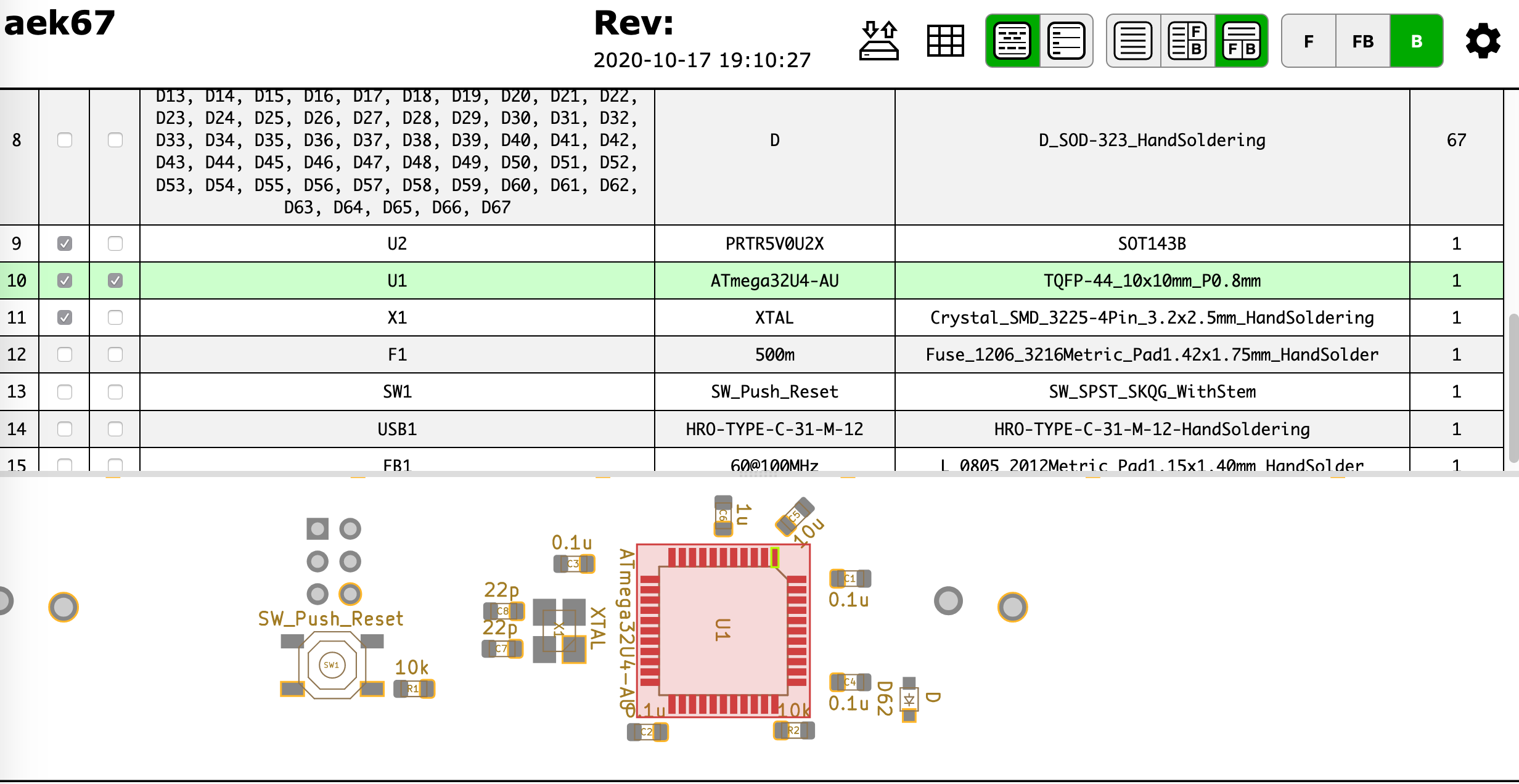
Notice that I selected the MCU. I can then see where the first pin is (it is outlined in flashy green), and how the MCU should be oriented.
So, I first add a bit of solder on pad 1 (top right in the picture) and another opposite pad:

Then I carefully place the MCU and reflow those pads to secure the MCU on the PCB (in the following picture it’s not that well placed, but I didn’t had a better picture):
The next step is to add flux on the pins:
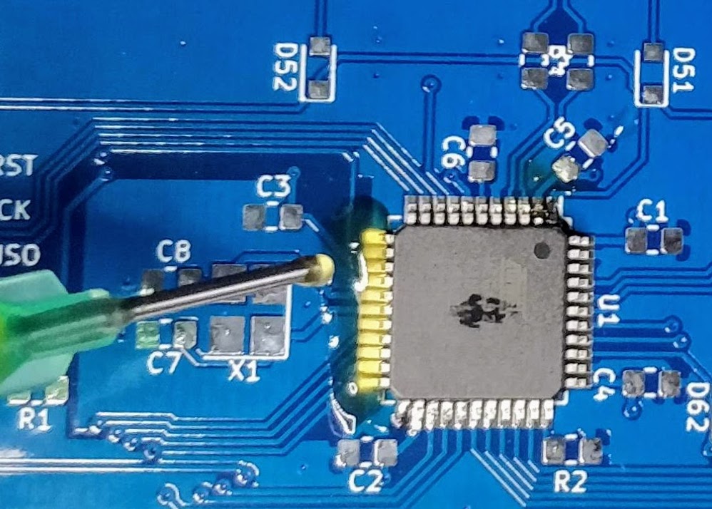
And drag soldering the left side:
Repeat the operation on the other three sides. Here’s a picture after soldering the whole component, but before cleaning the flux residues:

And a visual inspection with the magnifying glass:
So what to solder next:
F1Do not solder the diodes yet. It’s long and tedious, so it’s better to test the MCU works correctly before soldering them.
An advice when soldering is to sort the component bags in the order of the component you want to solder (following the interactive HTML BOM for instance). It’s very hard when looking at SMD components to identity them. Most of the time there’s nothing written on them, or if there’s something it’s not very helpful. That’s why I recommend to open the bag of the component that will be soldered only at the moment of soldering them. So the ritual is:
An alternative is to glue short sections of the components tapes on a cardboard board and tear apart the top tape when needed, then pick the components when ready to solder them.
Once all of the previously mentioned components have been soldered, it’s possible to test the PCB. Warning: do not connect yet the PCB to a computer. There could be a short circuit somewhere that could harm either the host or the keyboard (even though the host have some protections against those kind of failures).
Let’s see how to test the PCB with a multimeter. The first thing to check, is whether there’s continuity between the Vcc path, from the USB Vcc pins to the different MCU pins. If all Vcc pins are correct, check the GND pins. When all are correct, check there’s no continuity between GND and Vcc (at any point on the IC pins and USB pins). If that’s again fine, the next check is to make sure there’s no continuity between D+ and D- (this can be done at the USB connector).
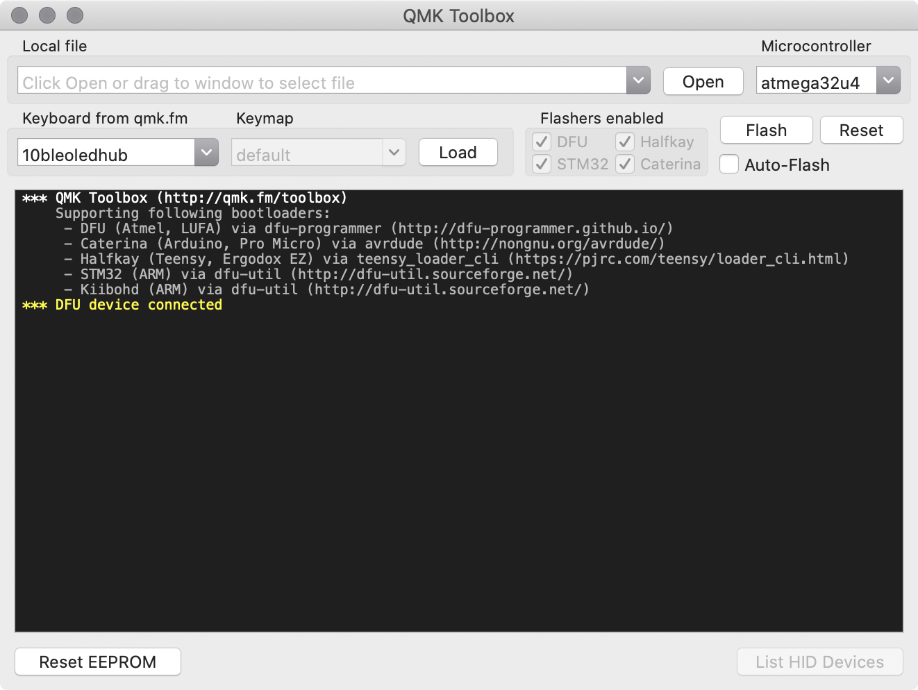
If everything is in oder, it is relatively safe to connect the PCB to a computer. Get an usb cable, then launch QMK toolbox. QMK Toolbox is a simple tool to help flashing QMK on a PCB. Once the keyboard is connected QMK Toolbox should display a yellow line indicating “DFU device connected” (at least for a DFU enabled MCU like our AtMega32U4):
If the test is conclusive, it’s time to solder the 67 diodes. Warning: diodes are polarized components, they need to be soldered with the correct orientation. A diode symbol looks like this:

One mnemotechnic way to remember which pin is what for a diode is to notice that the vertical bar and triangle form an inverted K and thus is the cathode, the triangle itself looks like an A (so is the anode).
On our schema and PCB, I’ve placed the cathode facing down:
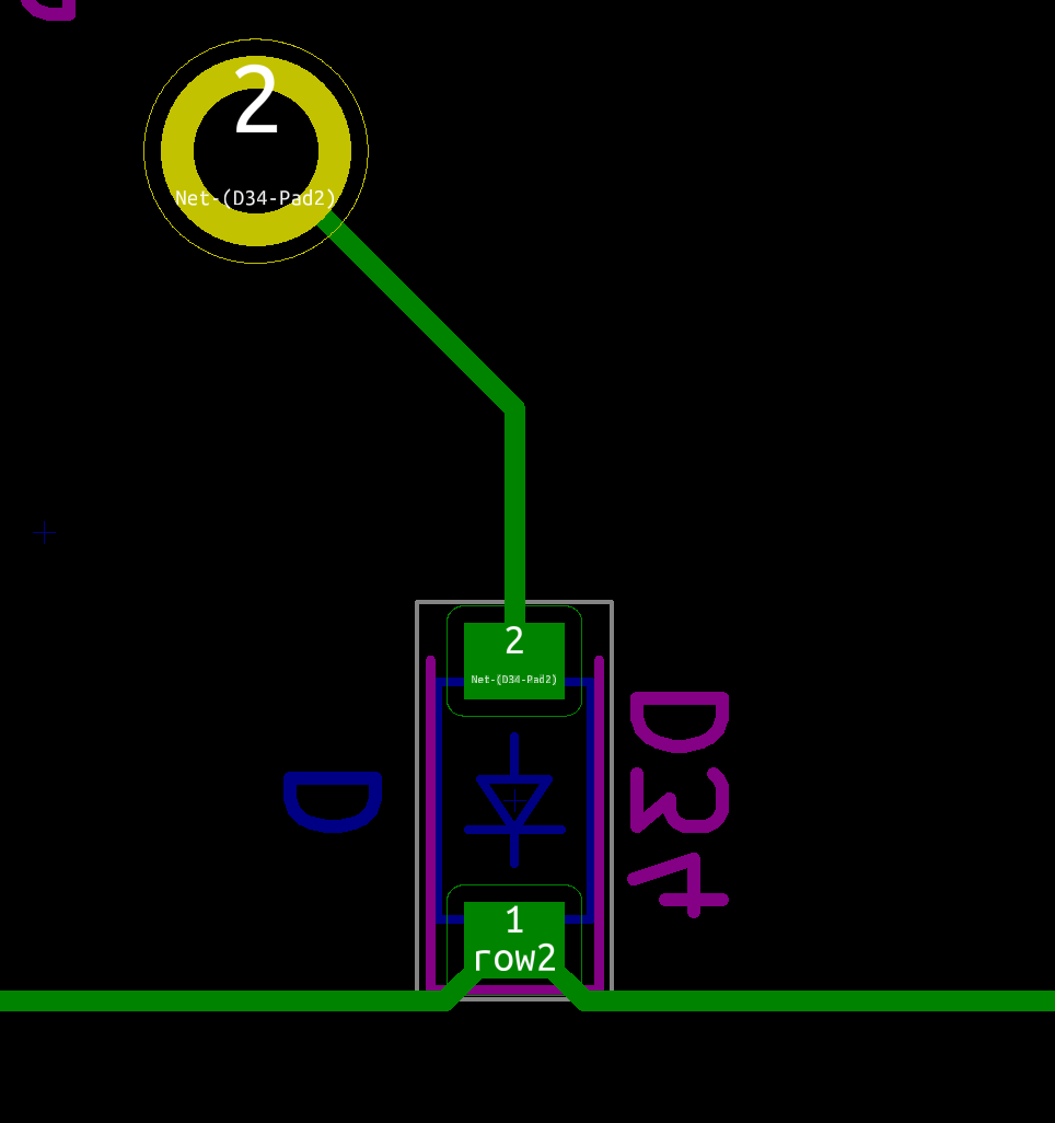
In Kicad, it’s easy to see the orientation of the diode because the B.Fab layer shows how to place it. On the manufactured PCB itself it’s not so easy as the fabrication layer is not shown. Instead we have a small horizontal bar to remind us where the cathode should be placed.
Hopefully the component itself also has a small bar printed on the top (here a close up of a 1N4148W-TP SOD-123, cathode on the left):
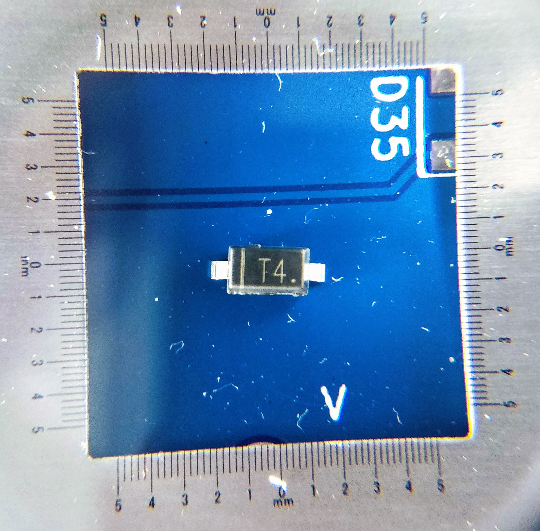
So to properly solder those diodes, it’s enough to align the component small bar with the bar printed on the PCB (which can partially be seen for the D35 diode in the image above).
The technique to solder a diode is the same as soldering any two pins SMD components. First add flux on both pads, add a small drop of solder on one of the pad, reflow it while holding the diode, then once solidified add a very small drop of solder on the other pad. Repeat for the 66 other diodes.
Here’s a soldered SOD-323 diode (smaller than the SOD-123 type we choose in this series of articles) :
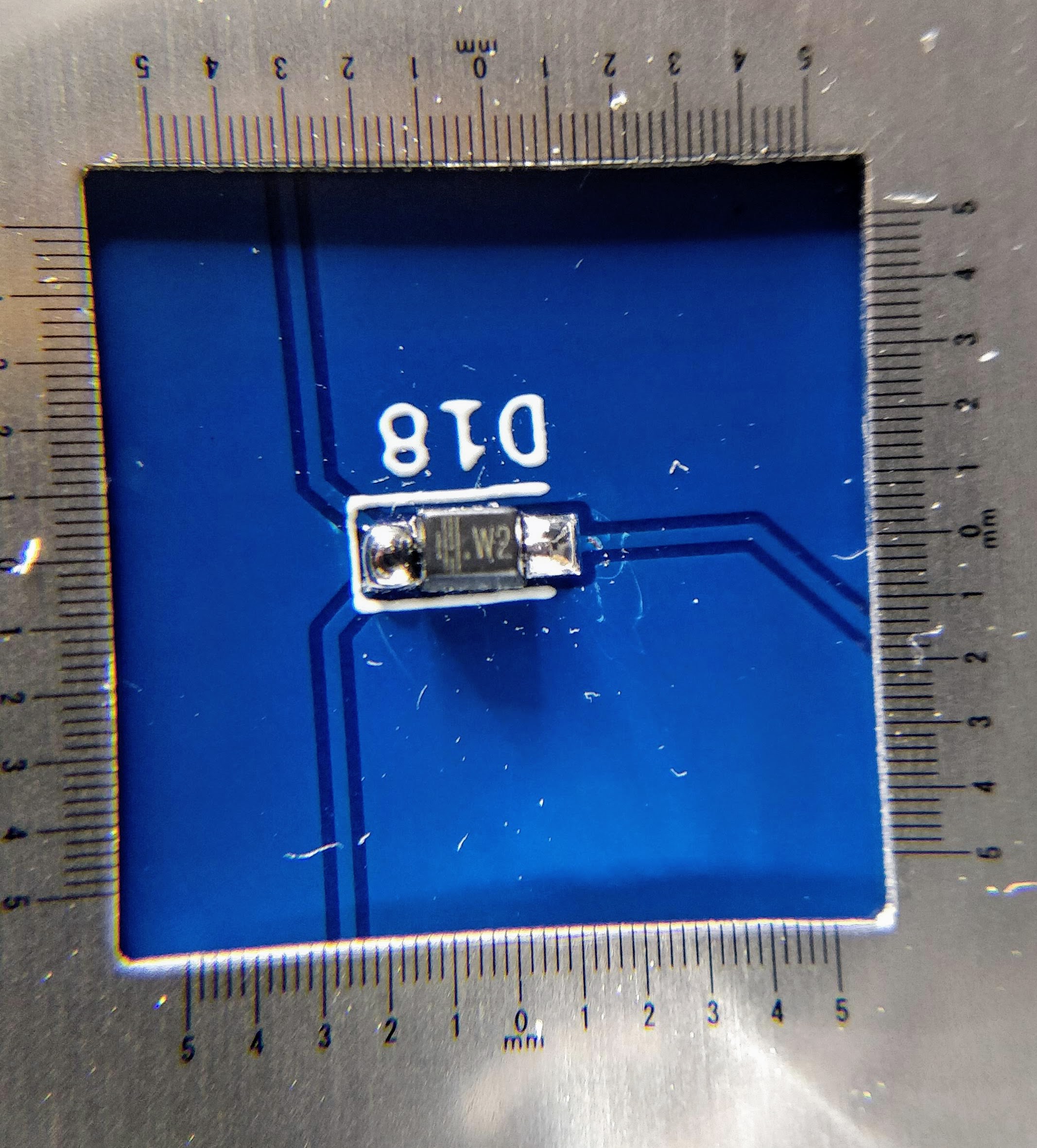
Once all the diodes are soldered, we can also check with the multimeter that they’re correctly placed and soldered. Again, if I put the multimeter in “diode testing” mode, put the red probe on the switch pin connected to the diode and the black probe on the MCU pin where the row is connected, the multimeter should display a diode forward voltage drop (around 650 mV). If it doesn’t then either the diode is placed in the wrong orientation or there’s a joint issue (that’s how I detected that I had inverted the diode for the P key). If that happens, you need to visually inspect the diode and joints.
To program the controller we’ll use QMK. This is an open source keyboard firmware forked and enhanced from TMK. It supports a miriad of custom keyboards and MCU (including various ATmega and ARM micro-controllers).
Follow QMK setup to install QMK and the needed toolchain on your computer.
Once done, check that you can compile a firmware, for instance the default DZ60 keymap:
% make dz60:default
QMK Firmware 0.11.1

Making dz60 with keymap default

avr-gcc (Homebrew AVR GCC 9.3.0) 9.3.0
Copyright (C) 2019 Free Software Foundation, Inc.
This is free software; see the source for copying conditions.  There is NO
warranty; not even for MERCHANTABILITY or FITNESS FOR A PARTICULAR PURPOSE.

Size before:
   text	   data	    bss	    dec	    hex	filename
      0	  23970	      0	  23970	   5da2	.build/dz60_default.hex

Compiling: keyboards/dz60/dz60.c                                                                    [OK]
Compiling: keyboards/dz60/keymaps/default/keymap.c                                                  [OK]
Compiling: quantum/quantum.c                                                                        [OK]
Compiling: quantum/led.c                                                                            [OK]
Compiling: quantum/keymap_common.c                                                                  [OK]
...
Compiling: lib/lufa/LUFA/Drivers/USB/Core/AVR8/USBController_AVR8.c                                 [OK]
Compiling: lib/lufa/LUFA/Drivers/USB/Core/AVR8/USBInterrupt_AVR8.c                                  [OK]
Compiling: lib/lufa/LUFA/Drivers/USB/Core/ConfigDescriptors.c                                       [OK]
Compiling: lib/lufa/LUFA/Drivers/USB/Core/DeviceStandardReq.c                                       [OK]
Compiling: lib/lufa/LUFA/Drivers/USB/Core/Events.c                                                  [OK]
Compiling: lib/lufa/LUFA/Drivers/USB/Core/HostStandardReq.c                                         [OK]
Compiling: lib/lufa/LUFA/Drivers/USB/Core/USBTask.c                                                 [OK]
Linking: .build/dz60_default.elf                                                                    [OK]
Creating load file for flashing: .build/dz60_default.hex                                            [OK]
Copying dz60_default.hex to qmk_firmware folder                                                     [OK]
Checking file size of dz60_default.hex                                                              [OK]
 * The firmware size is fine - 23816/28672 (83%, 4856 bytes free)
  5.37s user 4.17s system 82% cpu 11.514 total
You should obtain the dz60_default.hex file. You can remove it, it’s not needed.
QMK supports many keyboards and many layouts (called keymaps in QMK) for a given keyboard. A keyboard is defined by a directory in the keyboards/ folder, and each keymap is also a directory in the keymaps/ folder of a keyboard. To build such keymap, one need to use the make <project>:<keyboard>:<keymap> command.
The make command produces a hex file that can be flashed on the controller with QMK Toolbox, which is the recommended method. It is possible to flash from the command line depending on the controller bootloader type. I recommend QMK Toolbox because it is able to autodetect the correct bootloader, check the file size and so on. QMK Toolbox also acts as a console for the controller allowing to see debug statements.
Let’s bootstrap our new keyboard. Hopefully there’s a qmk command to do that:
% ./util/new_keyboard.sh
Generating a new QMK keyboard directory

Keyboard Name: masterzen/aek67
Keyboard Type [avr]:
Your Name: masterzen

Copying base template files... done
Copying avr template files... done
Renaming keyboard files... done
Replacing %YEAR% with 2020... done
Replacing %KEYBOARD% with aek67... done
Replacing %YOUR_NAME% with masterzen... done

Created a new keyboard called masterzen/aek67.

To start working on things, cd into keyboards/masterzen/aek67,
or open the directory in your favourite text editor.
This creates a set of files in keyboards/masterzen/aek67 that contains the default configuration for an AVR (ie AtMega) keyboard, including the default keymap:
% find keyboards/masterzen/aek67
keyboards/masterzen/aek67
keyboards/masterzen/aek67/aek67.h
keyboards/masterzen/aek67/config.h
keyboards/masterzen/aek67/keymaps
keyboards/masterzen/aek67/keymaps/default
keyboards/masterzen/aek67/keymaps/default/keymap.c
keyboards/masterzen/aek67/keymaps/default/readme.md
keyboards/masterzen/aek67/readme.md
keyboards/masterzen/aek67/aek67.c
keyboards/masterzen/aek67/info.json
keyboards/masterzen/aek67/rules.mk
I need to edit those files to map the hardware and matrix I created. Let’s start with the config.h file. This file contains the matrix description for this keyboard. We need to explain to QMK, what columns map to what pins on the MCU, and the orientation of the diodes. Based on our electronic schema, I can just write down the list of rows pins and columns pins:
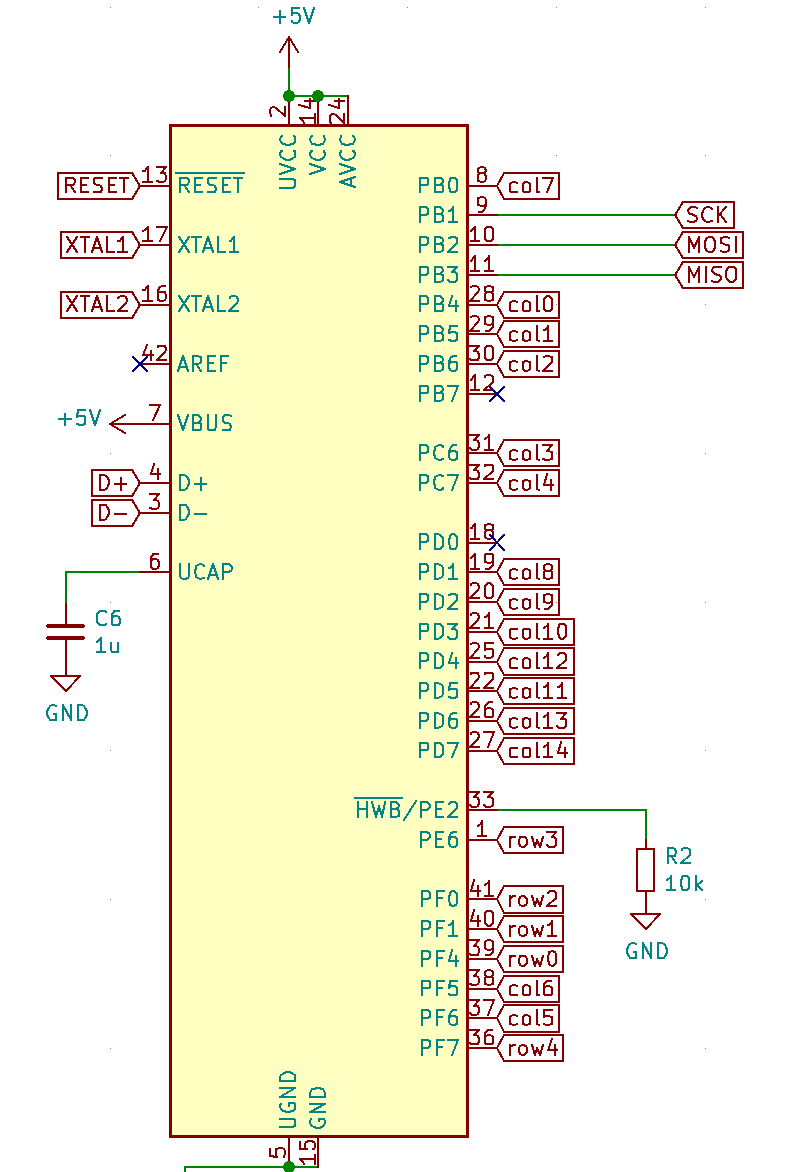
Here’s an extract of our config.h:
/* key matrix size */
#define MATRIX_ROWS 5
#define MATRIX_COLS 15

/*
 * Keyboard Matrix Assignments
 */
#define MATRIX_ROW_PINS { F4, F1, F0, E6, F7 }
#define MATRIX_COL_PINS { B4, B5, B6, C6, C7, F6, F5, B0, D1, D2, D3, D5, D4, D6, D7 }
#define UNUSED_PINS { B7, D0 }

/* COL2ROW, ROW2COL */
#define DIODE_DIRECTION COL2ROW
I defined here that the matrix is 5x15, and the ports of the rows and columns (in increasing order). Also, I tell QMK that the diodes are hooked between the columns and the rows (ie cathodes connected to the rows).
Next in rules.mk, we tell QMK everything about the controller used in this keyboard (there’s no need to edit anything there):
# MCU name
MCU = atmega32u4

# Bootloader selection
BOOTLOADER = atmel-dfu

# Build Options
#   change yes to no to disable
#
BOOTMAGIC_ENABLE = lite     # Virtual DIP switch configuration
MOUSEKEY_ENABLE = yes       # Mouse keys
EXTRAKEY_ENABLE = yes       # Audio control and System control
CONSOLE_ENABLE = no         # Console for debug
COMMAND_ENABLE = no         # Commands for debug and configuration
# Do not enable SLEEP_LED_ENABLE. it uses the same timer as BACKLIGHT_ENABLE
SLEEP_LED_ENABLE = no       # Breathing sleep LED during USB suspend
# if this doesn't work, see here: https://github.com/tmk/tmk_keyboard/wiki/FAQ#nkro-doesnt-work
NKRO_ENABLE = no            # USB Nkey Rollover
BACKLIGHT_ENABLE = no       # Enable keyboard backlight functionality
RGBLIGHT_ENABLE = no        # Enable keyboard RGB underglow
BLUETOOTH_ENABLE = no       # Enable Bluetooth
AUDIO_ENABLE = no           # Audio output
The next step is to define a key to matrix position mapping in aek67.h so that writing our keymap will be a bit easier:
...
#define LAYOUT_67_ansi( \
	K000, K001, K002, K003, K004, K005, K006, K007, K008, K009, K010, K011, K012, K013, K014, \
	K100, K101, K102, K103, K104, K105, K106, K107, K108, K109, K110, K111, K112, K113, K114, \
	K200, K201, K202, K203, K204, K205, K206, K207, K208, K209, K210, K211,       K213, K214, \
	K300, K301, K302, K303, K304, K305, K306, K307, K308, K309, K310,       K312, K313, K314, \
	K400, K401, K402,                   K406,                   K410, K411, K412, K413, K414  \
) { \
	{ K000,  K001,  K002,  K003,  K004,  K005,  K006,  K007,  K008,  K009,  K010,  K011,  K012,  K013,  K014 }, \
	{ K100,  K101,  K102,  K103,  K104,  K105,  K106,  K107,  K108,  K109,  K110,  K111,  K112,  K113,  K114 }, \
	{ K200,  K201,  K202,  K203,  K204,  K205,  K206,  K207,  K208,  K209,  K210,  K211,  KC_NO, K213,  K214 }, \
	{ K300,  K301,  K302,  K303,  K304,  K305,  K306,  K307,  K308,  K309,  K310,  KC_NO, K312,  K313,  K314 }, \
	{ K400,  K401,  K402,  KC_NO, KC_NO, KC_NO, K406,  KC_NO, KC_NO, KC_NO, K410,  K411,  K412,  K413,  K414 }  \
}
So the C macro LAYOUT_67_ansi contains 67 entries, one for each key, named by their rows and columns number (ie K204 is row2 and col4). This maps to a structure that represents the matrix in QMK (a double dimension array or rows and columns). Where the physical matrix has no switches (for instance in the bottom row before and after K406), we assign KC_NO so that QMK knows there’s nothing to be found there.
Next, let’s create the keymap. The keymap represents a mapping between the matrix switches and their functionality. When pressing a key, QMK will lookup in the keymap what keycode to send back to the computer. The computer will then interpret this keycode to a real character in function of the chosen layout. The keycode are defined by the USB HID standard. In QMK, they are defined as C macro whose name start with KC_. For instance KC_Q is the keycode for the Q key. See the QMK keycode table for an exhaustive list.
In QMK a keymap is a double dimension array of MATRIX_ROWS rows and MATRIX_COLS columns.
But that’s not the end of the story. QMK exposes different keymap layers. Layers are ways to assign multiple functions to a single key. We can assign a key in our keymap to switch to another layer where the keycode assigned is different than in the base layer. This is used for instance to map the function keys (F1 to F10) to the number keys.
Here’s the content of default/keymap.c:
enum layers {
    BASE,  // qwerty
    _FL,   // function key layer
};

/*
 * ,---------------------------------------------------------------------|
 * |`  |1  |2  |3  |4  |5  |6  |7  |8  |9  |0   |-   |=  |Backspace| PgUp|
 * |---------------------------------------------------------------------|
 * |Tab  |Q  |W  |E  |R  |T  |Y  |U  |I  |O  |P  |[  | ]  |   \     |PgDn|
 * |---------------------------------------------------------------------|
 * |Caps  |A  |S  |D  |F  |G  |H  |J  |K  |L  |;  |'  |  Enter     | Ins |
 * |---------------------------------------------------------------------|
 * |Shft    |Z  |X  |C  |V  |B  |N  |M  |,  |.  |/  |Shift       |Up| Del|
 * |---------------------------------------------------------------------|
 * |Ctrl|GUI |Alt |     Space                    |Alt |Fn  |  Lt |Dn |Rt |
 * `---------------------------------------------------------------------|'
 */
const uint16_t PROGMEM keymaps[][MATRIX_ROWS][MATRIX_COLS] = {
    [BASE] = LAYOUT_67_ansi(
        KC_ESC, KC_1,   KC_2,  KC_3,  KC_4,  KC_5,  KC_6,  KC_7,  KC_8,  KC_9,  KC_0,    KC_MINS,  KC_EQL,  KC_BSPC, KC_PGUP,
        KC_TAB, KC_Q,   KC_W,  KC_E,  KC_R,  KC_T,  KC_Y,  KC_U,  KC_I,  KC_O,  KC_P,    KC_LBRC,  KC_RBRC, KC_BSLS, KC_PGDN,
        KC_CAPS, KC_A,  KC_S,  KC_D,  KC_F,  KC_G,  KC_H,  KC_J,  KC_K,  KC_L,  KC_SCLN, KC_QUOT,           KC_ENT,  KC_INS,
        KC_LSFT, KC_Z,  KC_X,  KC_C,  KC_V,  KC_B,  KC_N,  KC_M, KC_COMM, KC_DOT,KC_SLSH,          KC_RSFT, KC_UP,   KC_DEL,
        KC_LCTL, KC_LGUI, KC_LALT,                  KC_SPC,                      KC_RALT, MO(_FL), KC_LEFT, KC_DOWN, KC_RGHT),

    [_FL] = LAYOUT_67_ansi(
        KC_GRV,  KC_F1, KC_F2, KC_F3, KC_F4, KC_F5, KC_F6, KC_F7, KC_F8,  KC_F9, KC_F10, KC_F11, KC_F12, KC_DEL, RESET,
        _______, _______, _______, _______, _______, _______, _______, _______, _______, _______, _______, _______, _______, _______, KC_HOME,
        _______, _______, _______, _______, _______, _______, _______, _______, _______, _______, _______, _______, _______, KC_END,
        _______, _______, _______, _______, _______, _______, _______, _______, _______, _______, _______, _______, KC_VOLU,_______,
        _______, _______, _______,                   _______,                            _______, MO(_FL), KC_BRID, KC_VOLD, KC_BRIU),
};
Notice a few things:
LAYOUT_67_ansi macro that I defined in aek67.h. This is to simplify using the matrix, because the matrix doesn’t have all the switches implemented.BASE and the so-called function layer _FL, that contains a few more keys._______ is an alias for KC_TRANS which means that this key isn’t defined in this layer. When pressing this key while being in this layer, the keycode that will be emitted is the first one to not be KC_TRANS in the layer stack. That means that Enter for instance is still Enter even for the _FL layer, but the up arrow key is volume up in the _FL layer.RESET key, so that it is easy to enter DFU mode to flash the keyboard (no need to open the case to get access to the hardware reset button)MO(_FL) is a special keycode that tells QMK to momentary switch to the _FL layer as long as the key id pressed. So activating RESET means maintaining MO(_FL) key and pressing the Page up key.Now let’s build the firmware:
% make masterzen/aek67:default
QMK Firmware 0.11.1

Making masterzen/aek67 with keymap default

avr-gcc (Homebrew AVR GCC 9.3.0) 9.3.0
Copyright (C) 2019 Free Software Foundation, Inc.
This is free software; see the source for copying conditions.  There is NO
warranty; not even for MERCHANTABILITY or FITNESS FOR A PARTICULAR PURPOSE.

Size before:
   text	   data	    bss	    dec	    hex	filename
      0	  18590	      0	  18590	   489e	.build/masterzen_aek67_default.hex

Compiling: keyboards/masterzen/aek67/aek67.c                                                        [OK]
Compiling: keyboards/masterzen/aek67/keymaps/default/keymap.c                                       [OK]
Compiling: quantum/quantum.c                                                                        [OK]
Compiling: quantum/led.c                                                                            [OK]
Compiling: quantum/keymap_common.c                                                                  [OK]
Compiling: quantum/keycode_config.c                                                                 [OK]
Compiling: quantum/matrix_common.c                                                                  [OK]
Compiling: quantum/matrix.c                                                                         [OK]
Compiling: quantum/debounce/sym_defer_g.c                                                           [OK]
...
Compiling: lib/lufa/LUFA/Drivers/USB/Core/AVR8/USBController_AVR8.c                                 [OK]
Compiling: lib/lufa/LUFA/Drivers/USB/Core/AVR8/USBInterrupt_AVR8.c                                  [OK]
Compiling: lib/lufa/LUFA/Drivers/USB/Core/ConfigDescriptors.c                                       [OK]
Compiling: lib/lufa/LUFA/Drivers/USB/Core/DeviceStandardReq.c                                       [OK]
Compiling: lib/lufa/LUFA/Drivers/USB/Core/Events.c                                                  [OK]
Compiling: lib/lufa/LUFA/Drivers/USB/Core/HostStandardReq.c                                         [OK]
Compiling: lib/lufa/LUFA/Drivers/USB/Core/USBTask.c                                                 [OK]
Linking: .build/masterzen_aek67_default.elf                                                         [OK]
Creating load file for flashing: .build/masterzen_aek67_default.hex                                 [OK]
Copying masterzen_aek67_default.hex to qmk_firmware folder                                          [OK]
Checking file size of masterzen_aek67_default.hex                                                   [OK]
 * The firmware size is fine - 16028/28672 (55%, 12644 bytes free)
  3.87s user 3.19s system 96% cpu 7.308 total
If it doesn’t compile, fix the error (usually this is a bad layer mapping, missing a comma, etc), and try again. The resulting firmware will be in masterzen_aek67_default.hex file at the QMK root.
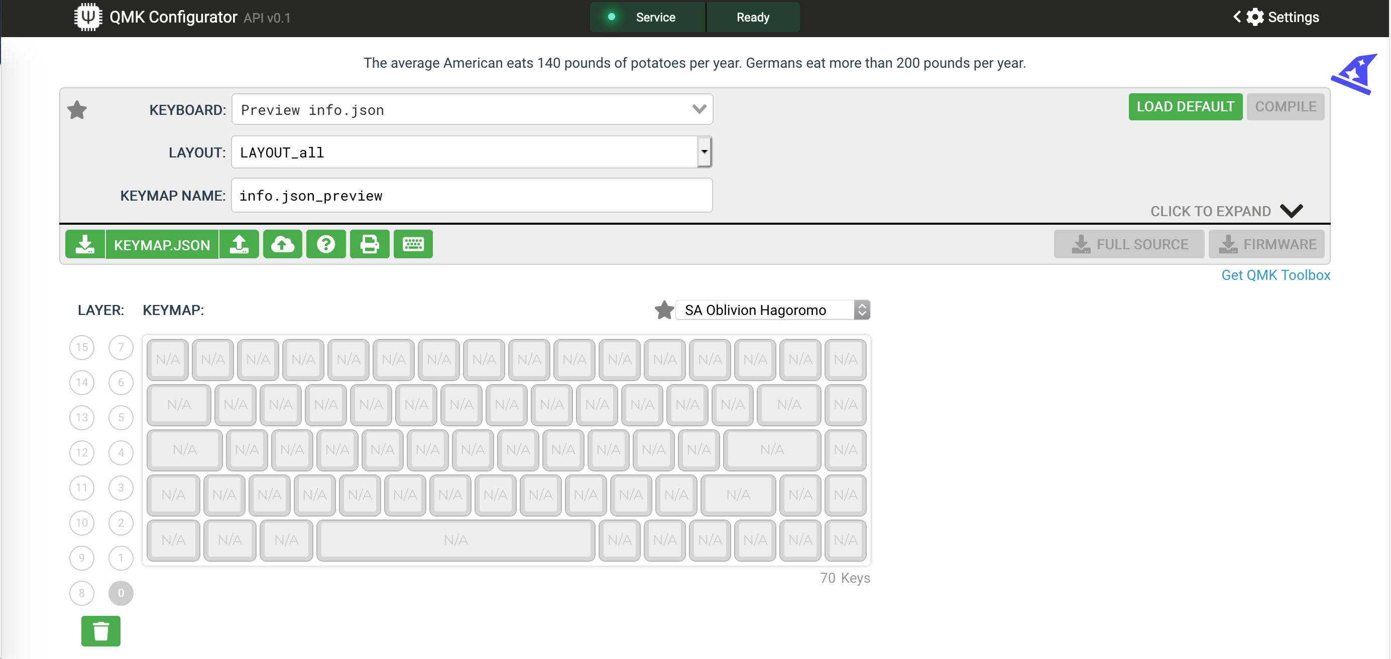
To properly finish the work, I also need to build a QMK Configurator json description file. This file tells the QMK Configurator how the keyboard looks (ie its layout) so it can display correctly the keyboard. It’s for people that don’t want to create their keymap in C like I did here. Producing this json file is easy to do from the Keyboard Layout Editor. Just copy the KLE raw content to a .txt file and run:
% qmk kle2json aek67-kle.txt
Ψ Wrote out info.json
It is possible to try the info.json file by going to the QMK Configurator and enter the Preview Mode by pressing Ctrl+Shift+i. This brings up a file selector window in which it is possible to open our info.json. If all goes well, the configurator will display the keyboard layout without any key label:
Finally, I can try to flash the firmware to the PCB:
*** Atmel DFU device connectedATMega32U4 microcontrollerYou should see something like this:
*** Attempting to flash, please don't remove device
>>> dfu-programmer atmega32u4 erase --force
    Erasing flash...  Success
    Checking memory from 0x0 to 0x6FFF...  Empty.
>>> dfu-programmer atmega32u4 flash --force /path/to/qmk_firmware/masterzen_aek67_default.hex
    0%                            100%  Programming 0x3F00 bytes...
    [>>>>>>>>>>>>>>>>>>>>>>>>>>>>>>>>]  Success
    0%                            100%  Reading 0x7000 bytes...
    [>>>>>>>>>>>>>>>>>>>>>>>>>>>>>>>>]  Success
    Validating...  Success
    0x3F00 bytes written into 0x7000 bytes memory (56.25%).
>>> dfu-programmer atmega32u4 reset
*** AtmelDFU device disconnected
At this point your computer should recognize that a new keyboard has been connected. If you press any switches it should produce a letter.
You can now test the keyboard and the keymap with the QMK Keyboard Tester. To do so, while the PCB is connected to the computer, use the tweezer to make contact between the two pins of each switch:
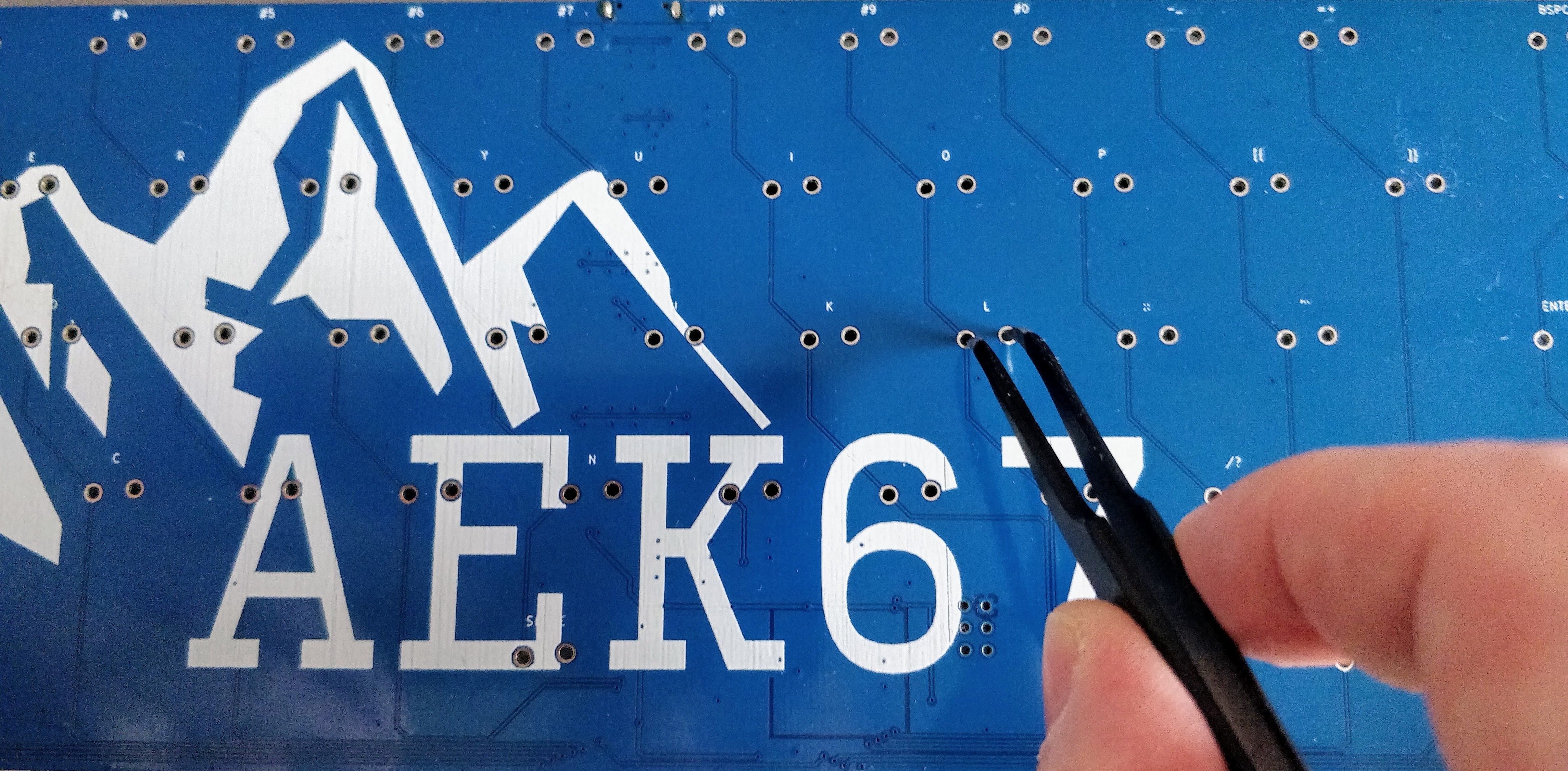
If the PCB and keymap are working correctly, the keyboard tester should display the key as registered:
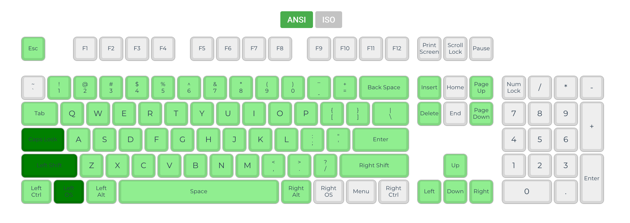
And voila, I now have a fully functional keyboard PCB!
And I think that episode concludes the series about keyboard PCB. I’ll expand soon the series of posts to talk about designing a nice case for the PCB.
I hope to be able to cover at least the following:
Thanks for following, and stay tuned for the next episodes!
Welcome for the third episode of this series of posts about designing a full fledged keyboard from scratch. The first episode focused on the electronic schema of the keyboard controller, the second one was on the components’ layout. In this one I’ll cover:
This is a long episode that took me a quite long time to produce. Feel free to leave a comment if you have any questions or find anything suspect :)
Routing is the process of connecting the various pins and pads of the circuits with copper traces while respecting the electronic schema. There are things that can and can’t be done for the PCB to be functional, for instance circuits have specific constraints for EMI, impedance matching, etc.
In the previous episode I decided to use a two layers PCB (which is the best compromise between cost and ease of routing for such projects). The switches are placed on the front layer, and because they are through-hole components they are being soldered on the back. All the rest of the components are laid out on the back of the board.
In the part 2 of this series of posts, I shown how to design the matrix schema. The matrix is a set of non-intersecting rows and columns. This means that if we were to route the matrix on the same PCB face we’d had an issue: all rows would collide with the columns.
Hopefully, since there are two layers in this PCB, I can route the columns on one side and the rows on the other side. Unfortunately there are other components to connect: the USB Type-C connector (and its ESD protection circuits), the MCU, the reset push-button, etc.
The USB Type-C connector is on the back layer at the top of the board, the MCU is also on the back layer but at the bottom. That means there are a few tracks to route vertically akin to the columns.
Inevitably some traces will intersect other traces. In such case it is possible to switch the trace to another layer by placing a via. A via is an electrical connection between two layers. The trace can then extend from one layer to another. Basically it is a hole that is metal plated to be able to conduct electricity. Note that there are different kinds of via, depending on if they cross the whole board or only some layers. In the case of two layers PCB, it will be through-hole vias.
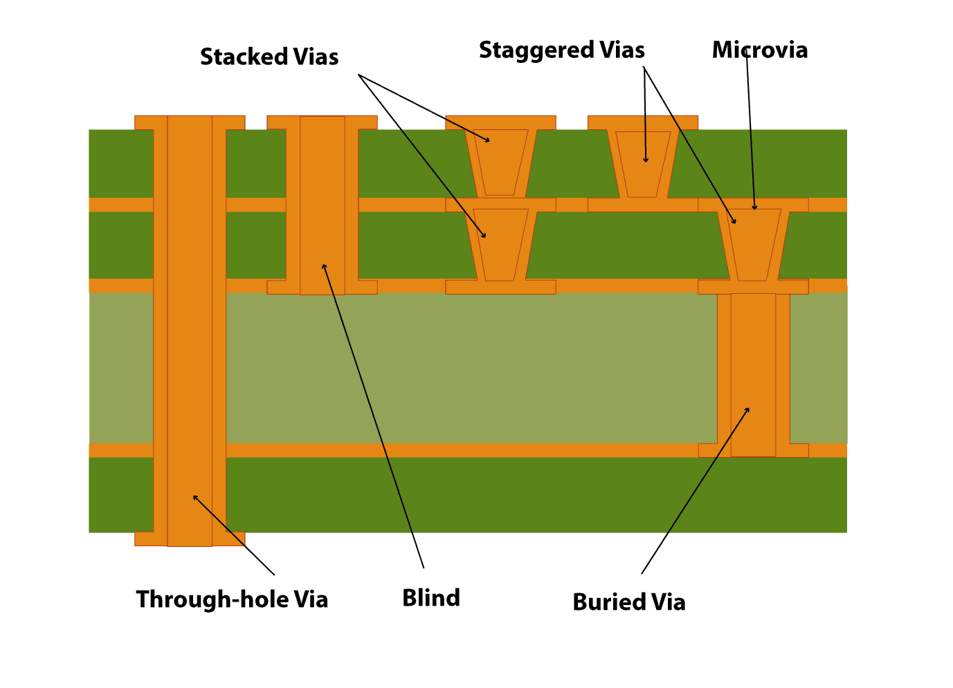
With a pair of vias in series the trace can jump to the other side and come back to its original side.
Another important thing to know is that a through hole pad (like the switch ones, but this is valid for any through-hole components) is available on both layers. This means a trace can piggy-back a switch pad to switch layer:
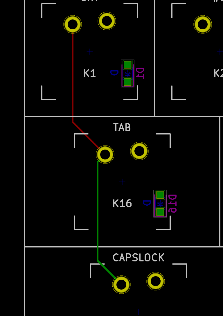
To prevent via abuse, the routing needs to take advantage of the number of layers. So for instance I can route the columns on the front layer, and the rows on the back layer.
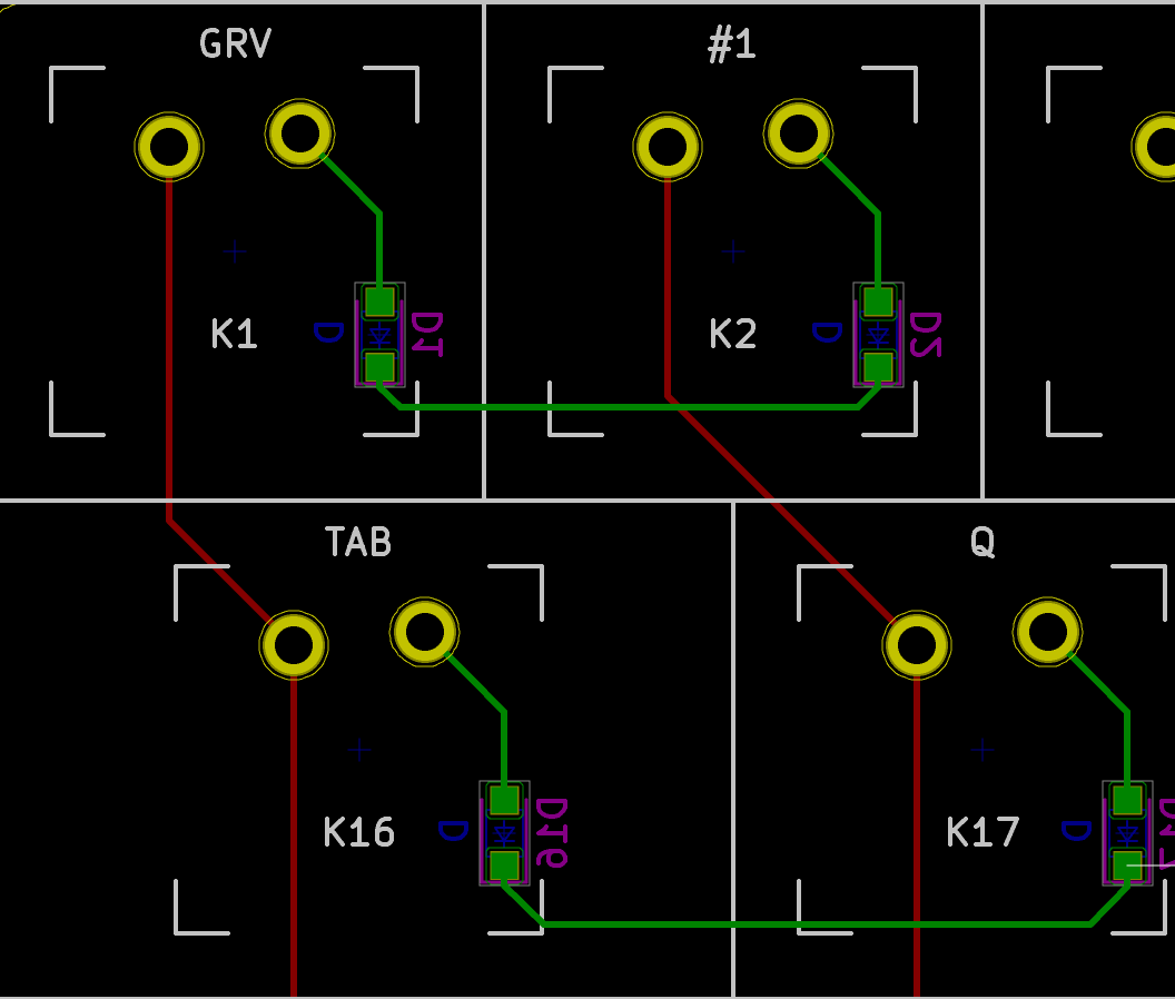
But it is also possible to do the reverse:
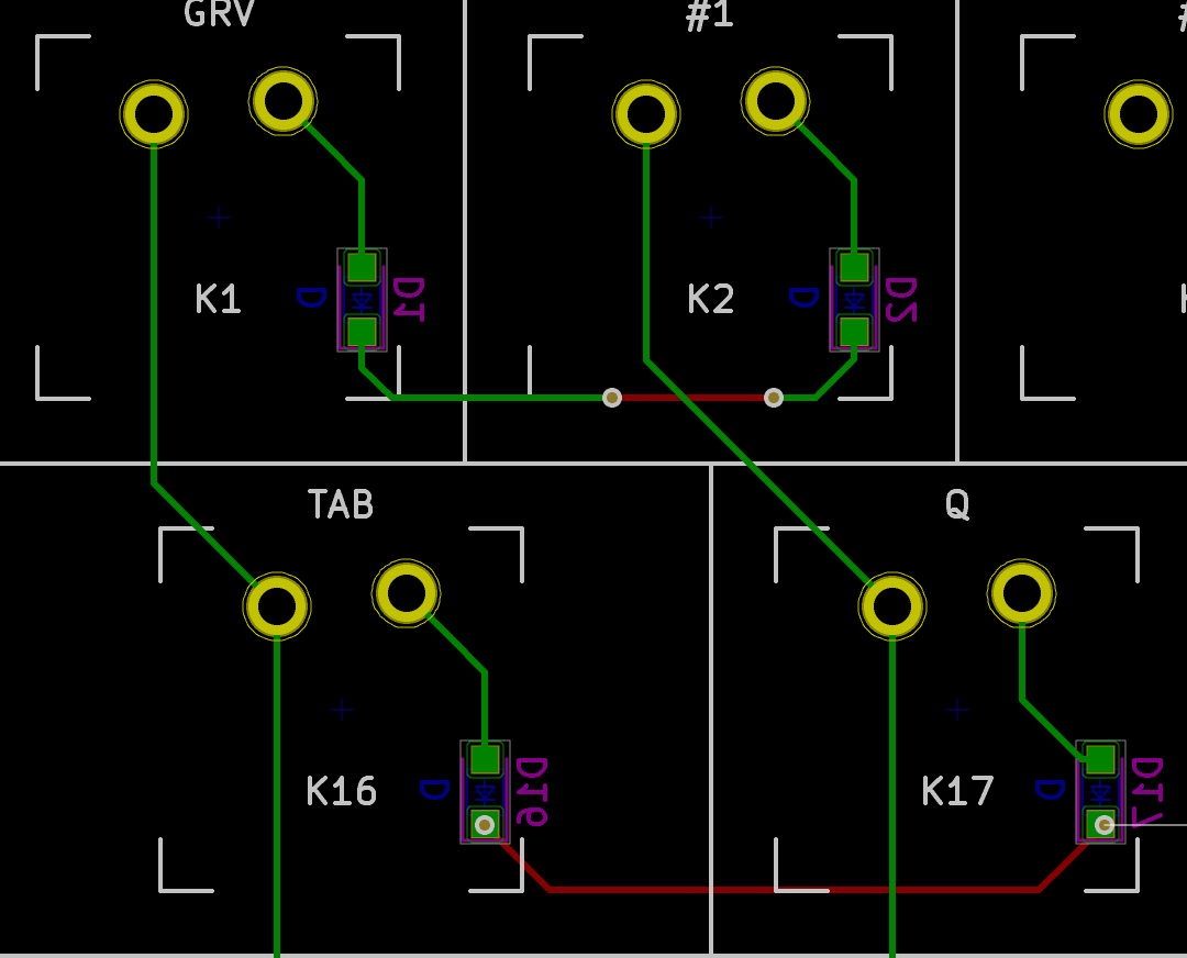
I was forced to use vias to jump other the column col1, because the diodes are on the backside. I tried two possibilities, using vias only for the minimal jump or using vias on the pad. Notice how both seems inelegant. Putting a via on a pad is also not a good idea unless the manufacturer knows how to do plugged vias. This can be needed for some high-frequency circuits where the inductance needs to be reduced. This isn’t the case of this very low speed keyboard, so I’ll refrain doing this.
Let’s route the columns. Start from the top left switch (or any other switch), then activate trace routing by pressing the x shortcut. Make sure that the F.Cu layer is active. If it’s not the case, you can switch from one layer to another by pressing the v shortcut. Caution: if you press v while routing a track, a via will be created. To start routing, click on the GRV left pad, then move the mouse down toward the TAB switch left pad (follow the net yellow highlighted line which shows where the net is connected):
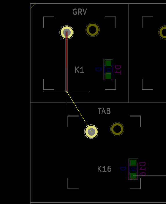
Notice that while routing a specific net, this one is highlighted in yellow, along with the pads that needs to be connected.
Keep going until you reach the next pad, and then click to finish the trace. Notice that the route is automatically bent and oriented properly. This is the automated routing:
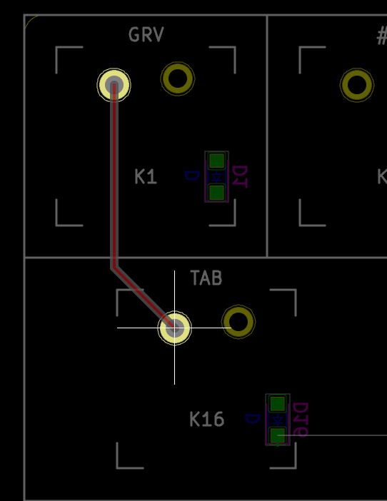
Keep going until all columns have been routed. Sometimes the trace is not ideally auto-routed by the automated routing system. In this case, it is possible to fix the problem by selecting the segment and use the Drag Track Keep Slope (shortcut d) to move the trace. For instance this trace pad connection could be made better :
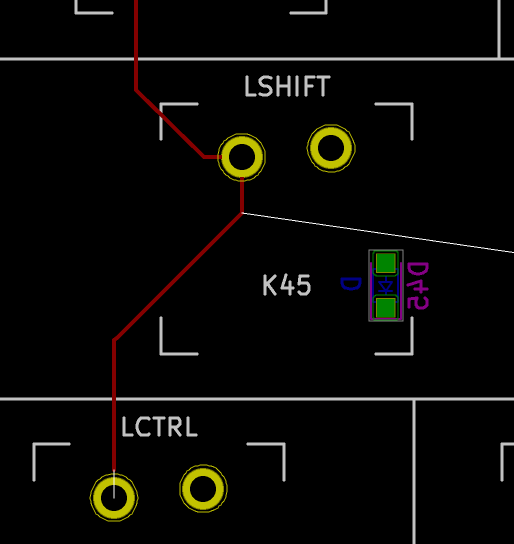
Dragging the track with d until I eliminated the small horizontal trace:
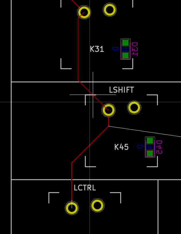
When all the columns are completed, the PCB looks like this:
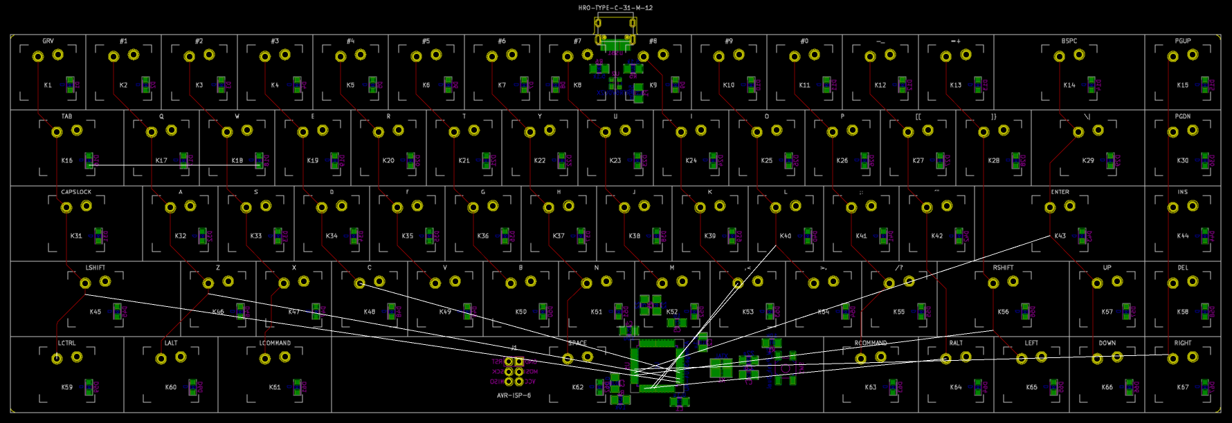
Notice that I haven’t connected the columns to the MCU yet, hence all the nets are directly linked to their assigned pads with those white lines.
Using the Show local ratsnest function we can highlight the columns nets, and verify that the connection scheme in part 2 is correct.
The idea was to have the columns on the extreme left or right be assigned the bottom part of the MCU (respectively left and right pads), and the center left columns (col5, col6) the left pads, the center columns col7 a free top pad, and the center right columns col8, col9 the right pads.
This gives this result:
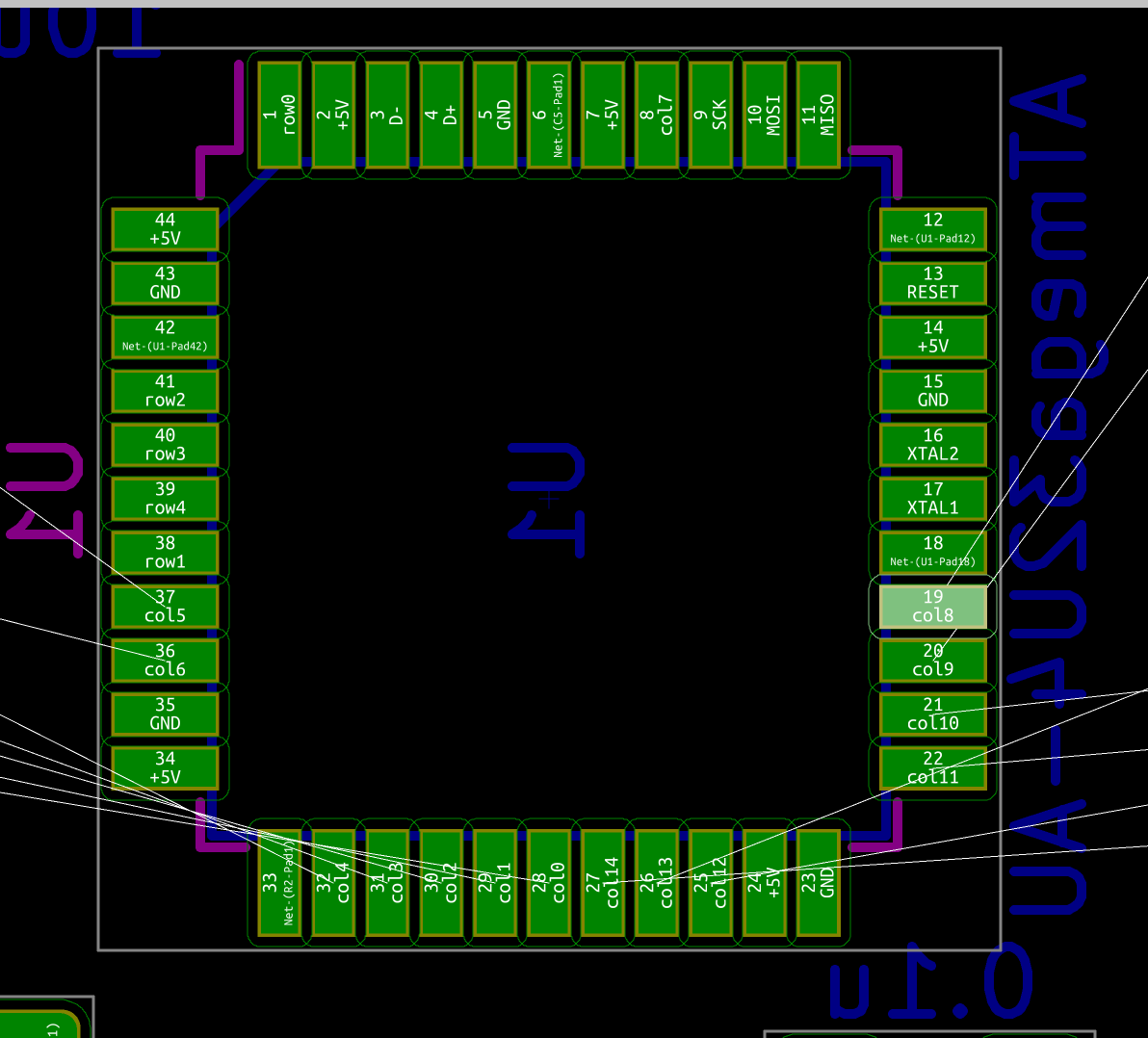
But before connecting the columns to the MCU, it’s better to route the USB data-lines and power rails.
The D+/D- USB data lines form what is called a differential pair. The idea is to send a complement signal on two wires instead of the normal signal on one. Traditionally a component uses GND as the reference for a signal in a single wire. This can be subject to EMI and noise. In a differential pair (and provided the impedance matches on both wire), the noise will affect both wire the same way. Since the MCU computes the difference between the two signals to recover the correct value, the noise is removed (because it is the same on both lines). The differential pair is thus much more immune to EMI and noise than a single trace.
Thus, differential pairs needs to be routed with care. Both trace needs to obey some important rules listed below.
To conserve coupling it’s best for the differential pair traces to keep their symmetry as good as possible.
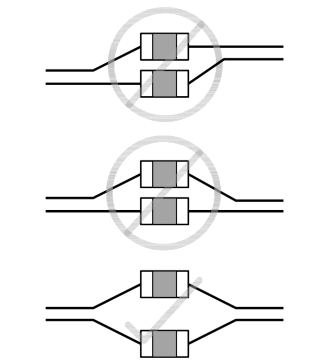
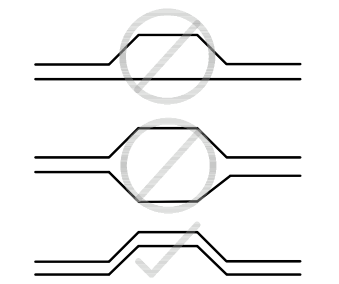
The noise-cancelling advantage of a differential pair works only if both signals arrive at the same time at the endpoint. If the traces have different lengths, one of the signal will arrive a bit later than the other, negating the effect. There’s a tolerance though, especially since this keyboard USB differential pair will run at the USB Full Speed standard (12 Mbit/s).
It’s possible to compute the time difference of the signals in function of the length difference. With the Full Speed standard a few centimeters difference will not incur a difference in arrival time, but this wouldn’t be true with high-speed signals. It’s best to keep the good practice of matching length all the time.
There’s no function in Kicad to check trace length, hopefully the trace length plugin can be used to check both traces length of the pair.
Obviously this will take less space on the PCB, which is good. But also the differential pair return current will flow in the ground plane below (if there’s one), possibly creating a current loop generating noise, if both tracks are not coupled enough because of their relative distance. This is again less an issue with USB Full Speed signals like the one this keyboard deals with (or with 2 layers boards without ground planes).
Each via adds inductance to the trace. It is usually recommended to not route those differential pairs through vias. But if vias have to be used anyway, make sure to use the same number of vias for both traces of the pair. With USB Full Speed signals, adding a few amounts of vias would probably not be detrimental, but it’s better to keep those traces on the same layer as much as we can as a good habit. Make sure to place all the IC so that there’s no need for differential pairs to change layers. That’s also the reason differential pairs should be routed first.
The differential pair should not be too close to other signals or other differential pairs. A good rule of thumb is to apply a spacing of 5 times the trace width (this is known as the 5W rule).
Where the differential pair comes close to high speed signals (for instance clock traces), the spacing must be increased again (for instance 50mils). Differential pairs should also be spaced from other differential pairs to prevent cross-talk (use the same 5W rule).
Spoiler alert: all circuits form a closed loop. The signal in a differential pair is a current that needs to flow back to it’s source at some point. At higher frequencies, the return current will follow the lowest impedance path. This usually happens to be the closest reference plane (a ground or power plane if there’s one). If there’s a void or a split in the reference plane, the return current will have a longer path leading to excess electromagnetic emissions, delayed signal, etc.
The differential pairs should not be routed under or near a crystal oscillator or resonator.
When a single track or another differential pair crosses (on a different layer) a differential pair, do it with an angle of > 30º and < 150º to minimize cross talk. To make it more easy target 90º intersections.
A stripline is a layer trace embedded in a dielectric medium itself sandwiched by two copper plane. On the reverse a microstrip is a trace at the surface (not embedded). It’s best to route differential pairs as microstrips.
If possible, the differential pair should never do a straight U-turn. When bending, maintain a 135º angle all the time.
The recommendation is to keep at least 90mils between the traces and the ground plane edges.
The USB 2.0 standard requires the transmission lines (ie cables and connected PCB tracks) to have a differential impedance of 90 ohms (which translate to a single line impedance of 45 ohms) +- 10%.
Maintaining the impedance is capital to prevent high frequency signals to bounce. To perform controlled impedance routing, you need to compute the single trace width and spacing (there are calculators online and even one in Kicad; the free Saturn PCB calculator is a good reference but works on Windows only).
It’s relatively easy to control the impedance if there’s a continuous ground plane not far below the tracks (so it’s best to route those on 4+ layers PCB). But for a 2-layers PCB, assuming one of the layer is an uninterrupted ground plane, the trace size would have to be 38 mils spaced with 8 mils to match the 90 ohms impedance. This is because the height of the dielectric board is around 1.6 mm for a 2 layers board, whereas it is less than a 1 mm between two copper layers on the same side of the board.
Hopefully, if our traces are shorter than the signal wavelength there’s no need to implement controlled impedance. With a tool like the Saturn PCB Calculator we can estimate the USB Full Speed wavelength and thus our max trace length.
The USB Full Speed rise time is between 4 ns to 20 ns. When injecting the worst case of 4 ns in the Bandwidth & Max Conductor Length calculator, the result is a bit more than 18 cm. Since this keyboard is currently 9.5 cm wide and the USB D+/D- will be traced as straight as possible, the differential pair length will be well within the safety margin. Based on this, I’m going to use 10 mils as trace width and spacing.
Stubs should be avoided as they may cause signal reflections. For USB, this is seldom a problem as the data traces are point-to-point.
Most of these recommendations were gleaned from TI High-SpeedLayoutGuidelines, Silicon Labs USB Hardware Design Guide, Atmel AVR1017: XMEGA - USB Hardware Design Recommendations, Intel EMI Design Guidelines for USB Components. I also recommend reading Eric Bogatin - Signal and Power Integrity - Simplified and Henry W. Ott - Electromagnetic Compatibility Engineering. Refer to those documentations for more information.
Now let’s apply this knowledge to this keyboard. First I need to prepare the USB connector data lines: since there are 4 pads for the two datalines (to support reversibility) they need to be connected together:
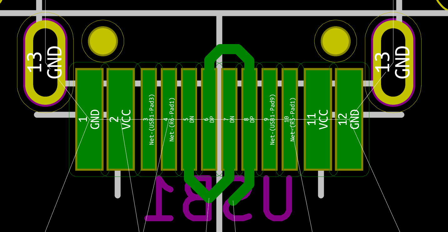
Use the Route → Differential Pairs feature and start laying out the traces from the connector. Uh oh, an error pops-up:
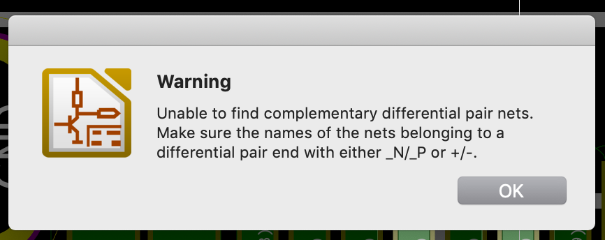
To be able to route a differential pair, Kicad requires its nets to obey a specific naming. Net names should end up in P/N or +/-, which is not the case here. The USB pads nets have no name, as they acquire their name only after the impedance matching resistors. To correct this, I just need to assign name to the wires in the schema editor:
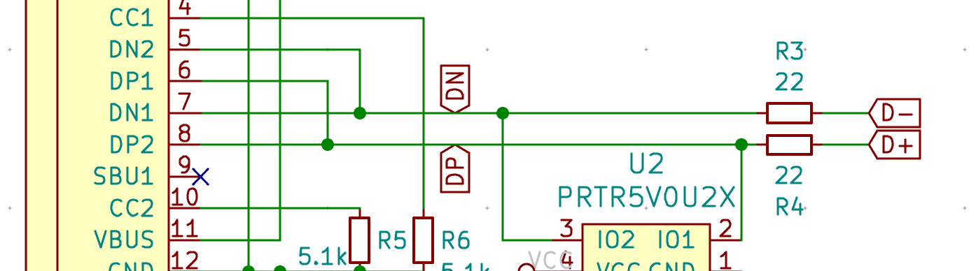
And finally using Update PCB from schematics, I can start routing the USB data-lines (using the Route → Differential pair function):
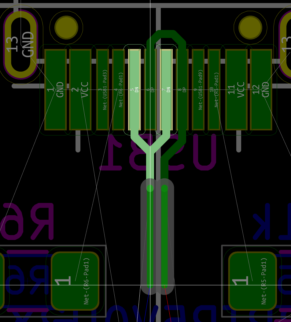
The next step is to connect the differential pair to the PRTR5V0U2X. Unfortunately Kicad is not very smart when connecting a differential pair to pads. It’s better to stop drawing the differential pair, switch to single track routing mode and connect the pads to the differential pairs. Since it’s important to minimize stubs, it’s best to uncouple a bit the differential pair to connect it to pads, like this:
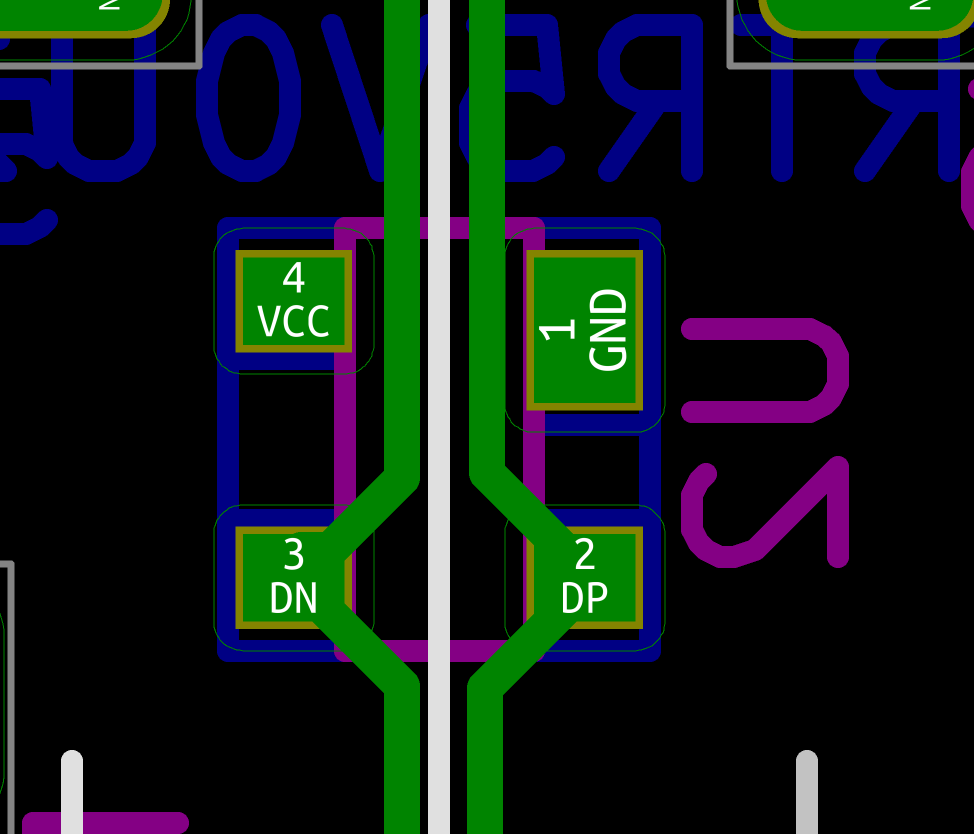
Then, the differential pair can be routed to the pair of impedance matching resistors (which are located close to the MCU):
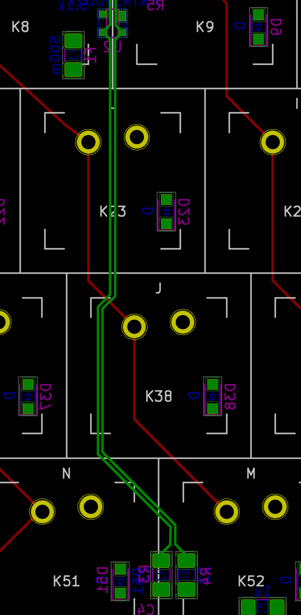
To connect the resistors to the MCU with a differential pair, it’s easier to start from the MCU by using the Route → Differential Pair function and connect the MCU pads to the resistors pads:
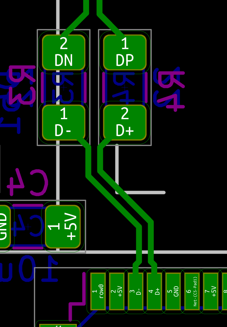
Now, I can check both trace lengths with the Measure Length of Selected Tracks plugins. To do that, select one trace of the pair, and use the u shortcut to select it fully. In the case of this keyboard, I got 70.05 mm for the left traces and 69.90 mm for the right one. This is small enough to not try to optimize it.
The final routing of this differential pair looks like this:
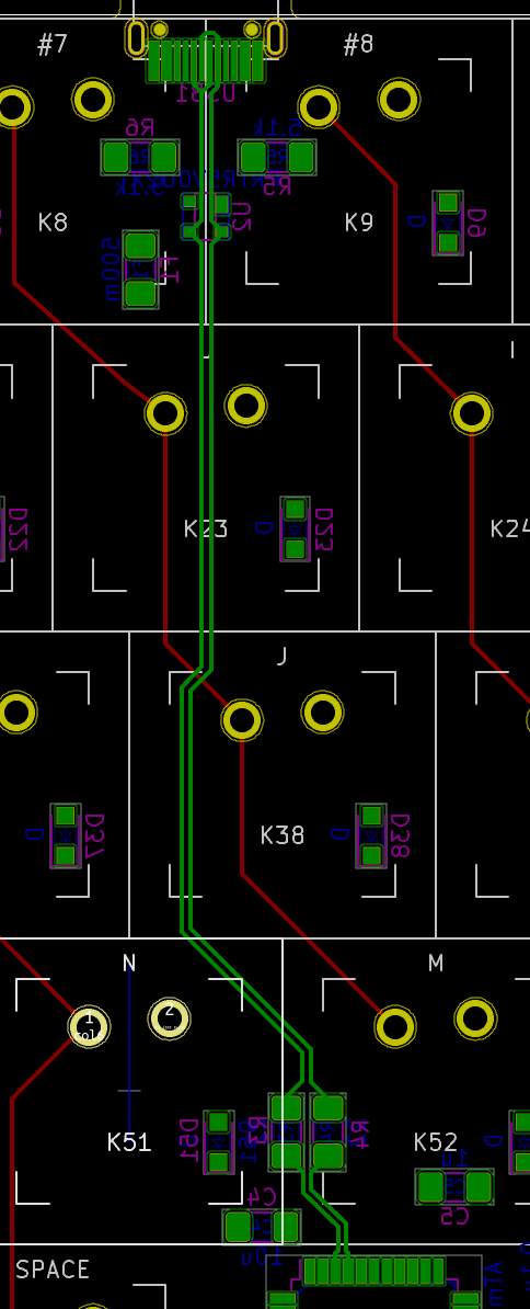
The first step is to connect the right switch pad (#2) to its diode anode for every switch:
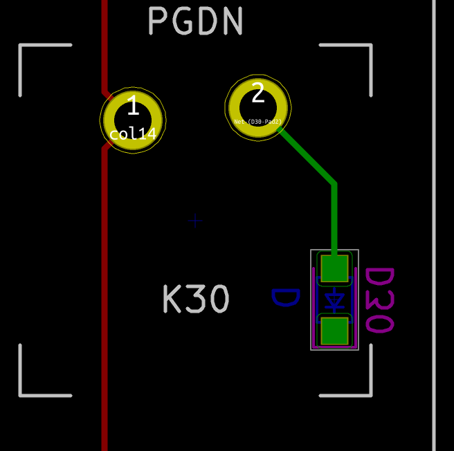
Then connect all cathodes together with a track forming the row. Draw a straight line first:
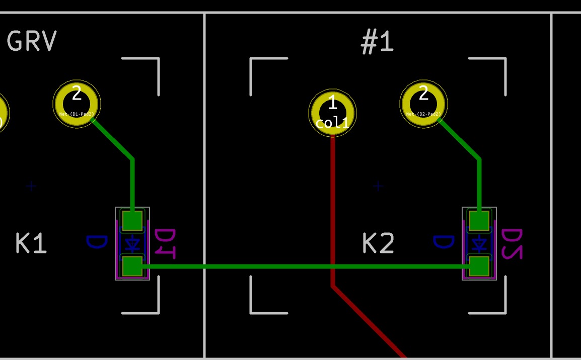
Then use the d shortcut to produce a more appealing form by dragging the track toward the bottom:
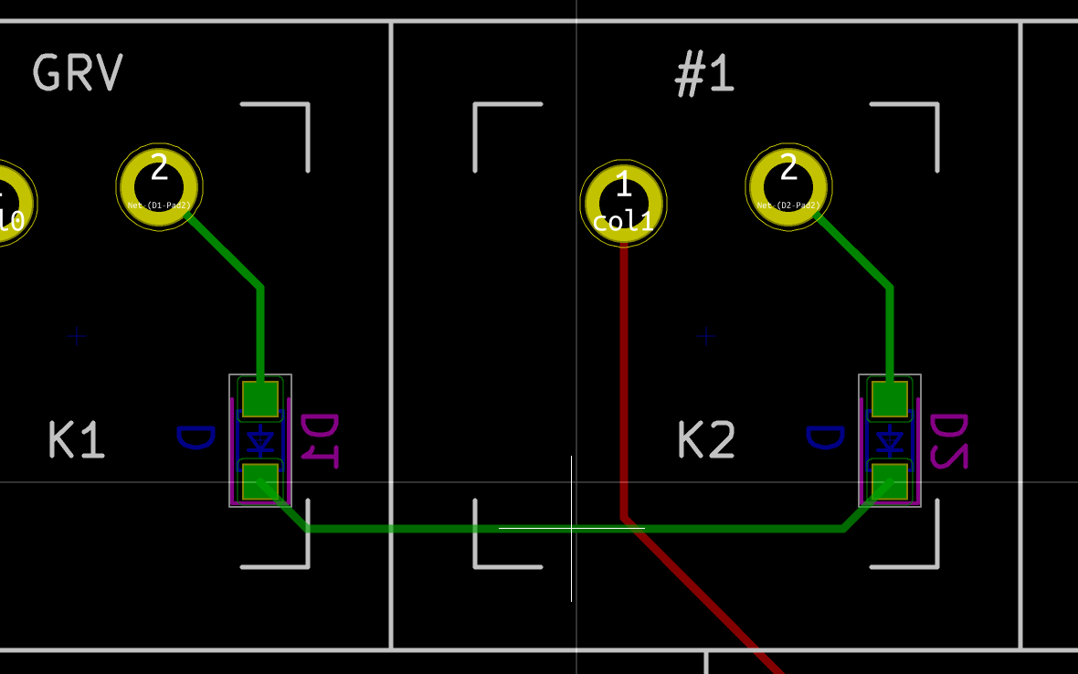
Do that for all the switches, but do not connect the rows to the MCU, nor cross the USB differential pair yet, because there will be some choices to be made and experimentation.
Routing the crystal oscillator is easy as there are few tracks and components. The crystal generates a square wave signal at 16 MHz. A square signal is the combination of a lot of powerful harmonics in the frequency domain. Those are an issue for EMC, so special care has to be applied for placement and routing of the clock circuits.
The first rule is that we have to make the XTAL1 and XTAL2 trace as short as possible. This means the crystal has to be as close as possible to the MCU, this is in order to minimize parasitic capacitance and interferences. For the same reason, avoid using vias in the crystal traces.
The second rule is that we have to space other signals as much as possible to prevent the clock noise to be coupled to other traces (but also the reverse). To prevent as much as possible this effect, it is recommended to add a GND guard ring around the crystal traces.
The main problem with crystal oscillators is the return current. Every electrical circuit form a loop, so the current that gets in the crystal, needs to go back to somewhere for the crystal oscillator to work. This return current is also a square signal containing high frequency harmonics. The problem is that the loop formed to return the current is a kind of antenna. If it is large, it will radiate a lot of EMI which we want to minimize (and also if it’s an antenna it will be susceptible to external emission which we also want to minimize). I’ve seen design with a general ground and vias connected to the crystal GND: in such case this pour becomes a nice patch antenna. If we were to design this keyboard with a ground pour, the one under the crystal oscillator should be an island not connected to the rest of the ground pour to prevent radiating everywhere and to make sure the current return loop is as small as possible. In fact, it’s even better to add a ground pour guard ring on the same layer as the crystal (the loop formed in this case will be shorter than crossing the 1.6 mm PCB dielectric).
The 22pF load capacitors should be placed as close to the crystal as possible.
Let’s start by connecting the crystal oscillator to the MCU (both XTAL1, XTAL2 and GND):
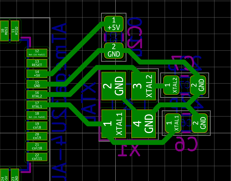
Then using the Add Filled Zone tool (select the GND net), we’re going to draw a rectangle around the crystal:
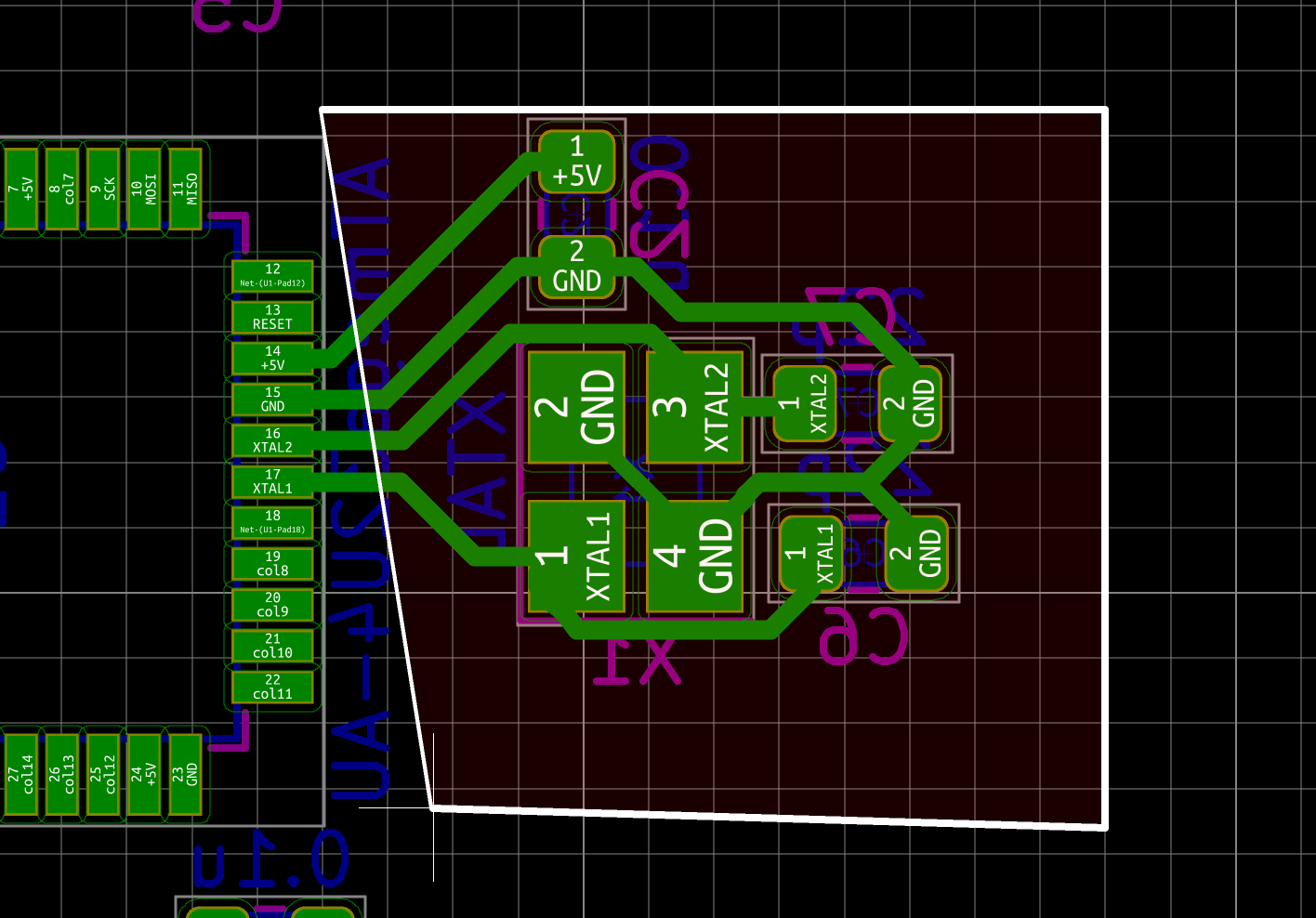
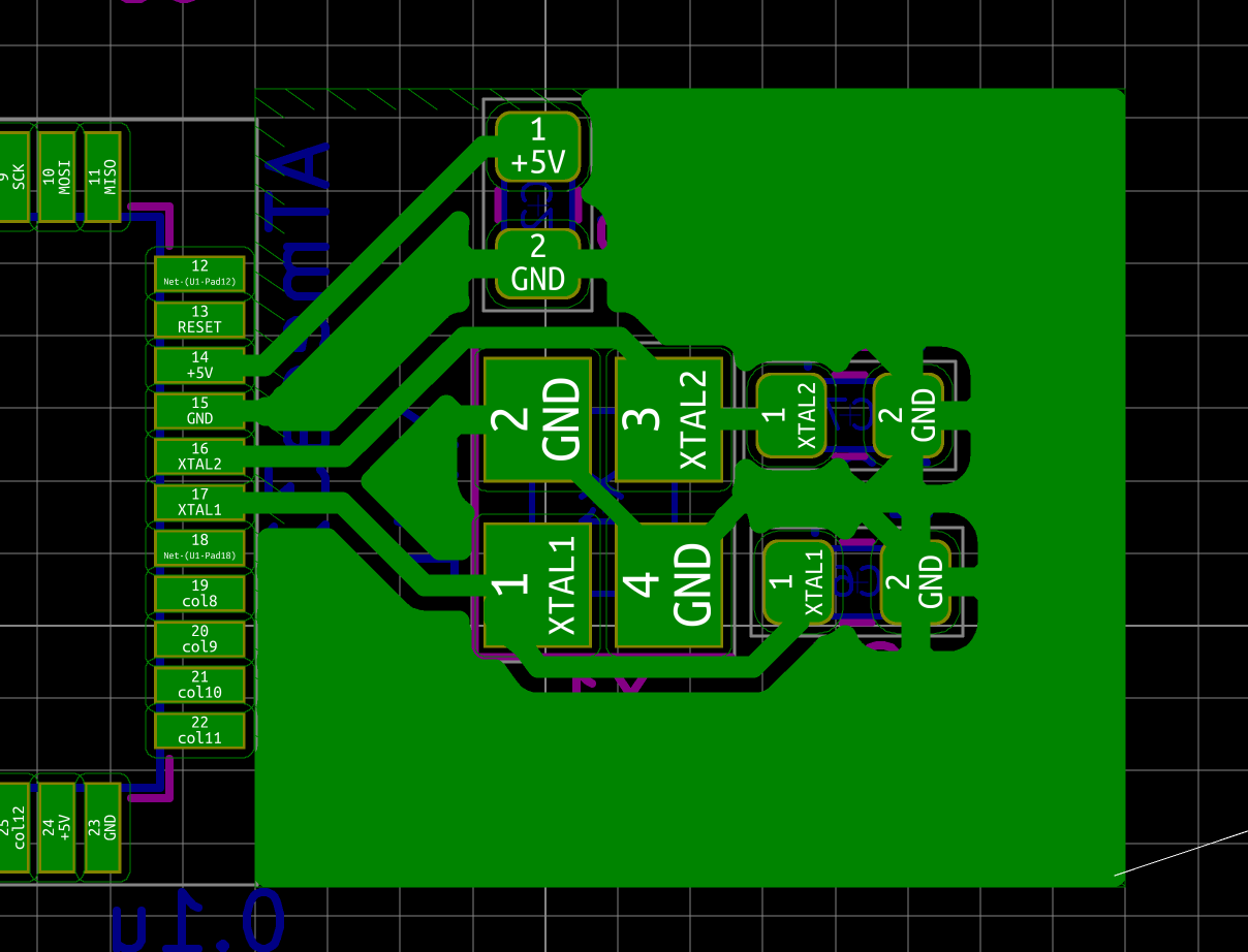
If we want to add a copper ground island in the other layer (F.Cu), we can do this easily by right clicking one of the control point of the filled zone we just added and use Zones → Duplicated Zones onto layer, then select F.Cu. This zone will not be connected to anything, so we have to add a few vias:
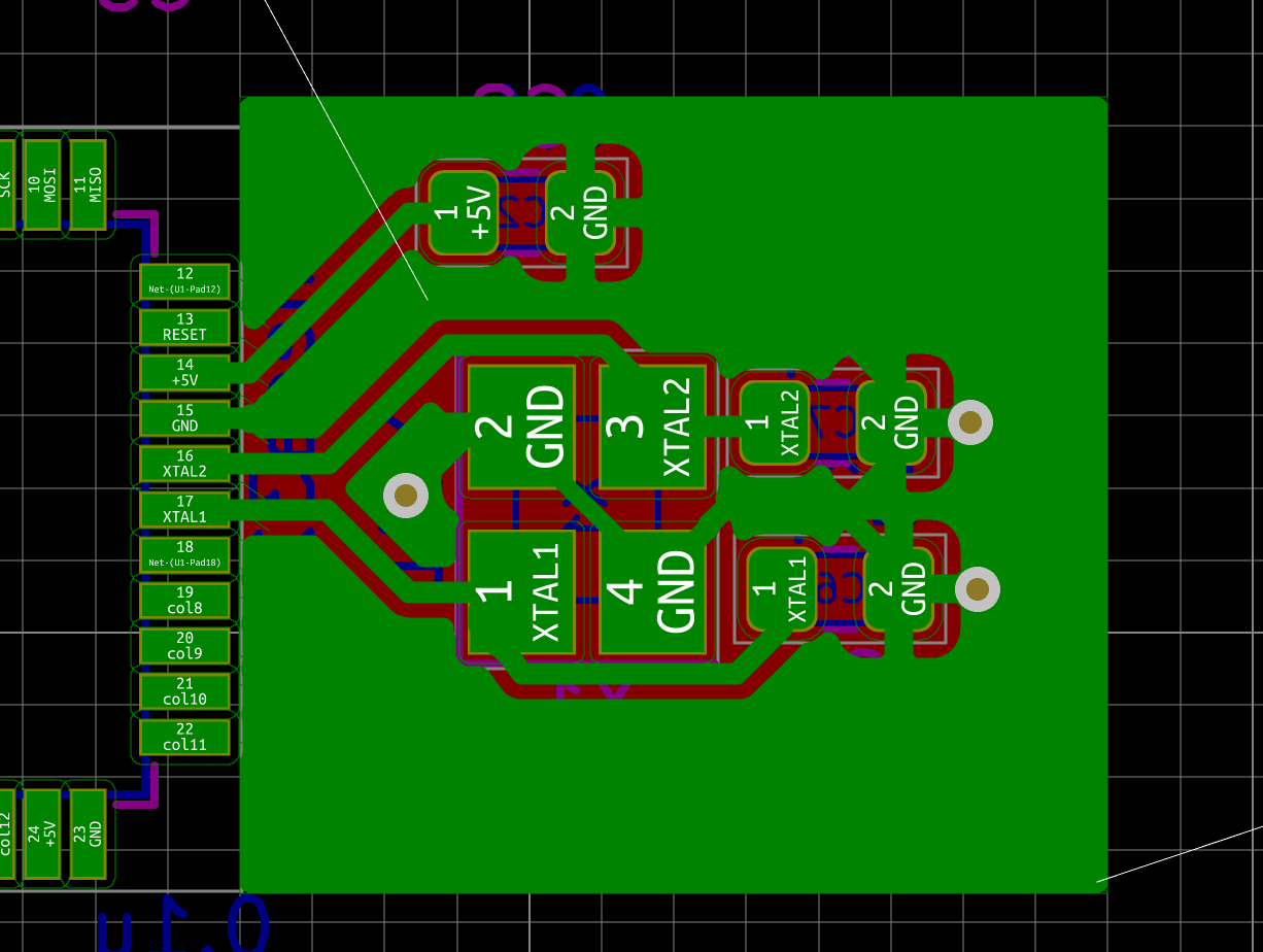
This isn’t complete, we should probably extend the underlying zone under the XTAL1 and XTAL2 MCU zone. First select the F.Cu layer, then right-click on the Create Corner function to add a control point. Do it again and extend the zone under the GND, XTAL1 and XTAL2 pads:

The next thing to do is to power the active components. It’s always best to route power and ground traces before the signal traces. Our signal traces can be moved around, they are not critical and are narrower than power traces.
Hopefully there’s only one active component in this keyboard the MCU (keyboards with leds, underglow rgb, rotary encoder might have more than one active component). The power comes from the USB port delivered directly by the host.
The first step is to wire the USB Type-C power traces (and also the CC1 and CC2). There are several possibilities, depending on where we want the +5V and GND to come from (since there are 2 pads with those nets on the USB connector to support both orientations).
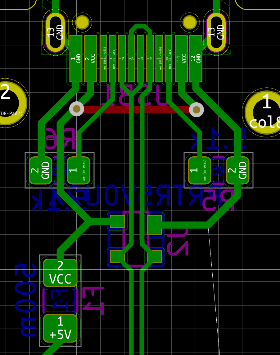
Notice that I haven’t yet wired GND. Then I can route +5V down to the MCU. I deliberately spaced the trace from the D+/D- USB differential pair to prevent it to couple into the power trace (remember the 5W rule from earlier?)
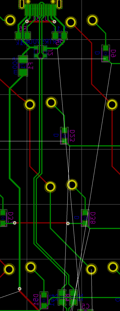
This power trace needs to deliver power to all the VCC pads of the MCU. The best way to do that is to use a grid system around the MCU on the other layer. Do not close the loop, that would be quite bad.
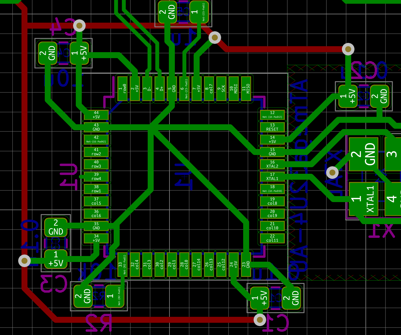
At the same time I connected the GND pads together with a kind of badly shaped star. I’ll replace it with a local ground pour, but if not, the star would have to be redesigned to have less acute angles. There’s an interest in having a ground pour behind the MCU (on the same layer), it will help conduct the generated heat and serve as a poor’s man radiator.
Even though I’ll use a ground pour on the front and back layer, it’s better to materialize the GND trace to the MCU. If possible I’ll come back and simplify the routing when those pour will be laid out. Meanwhile, the PCB would still be functional:
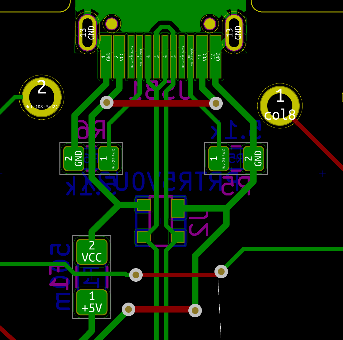
Then route the GND trace close to the +5V one down to the MCU:
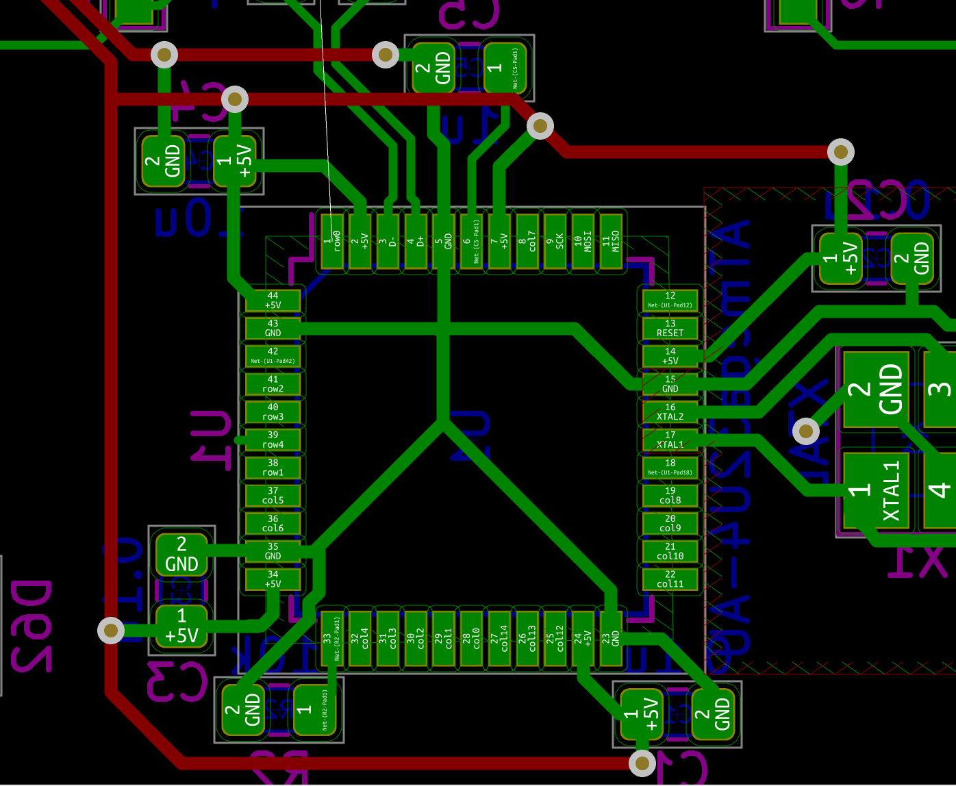
Make sure to not create any GND loops.
I’m going to connect the matrix. This will also allow checking if the projected connection scheme on the MCU will work or not.
I’m used to starting from the MCU and progress toward the matrix rows and columns. A good way to do that, is to start some kind of bus from the MCU pads going globally in the direction of the rows or columns to connect like this:
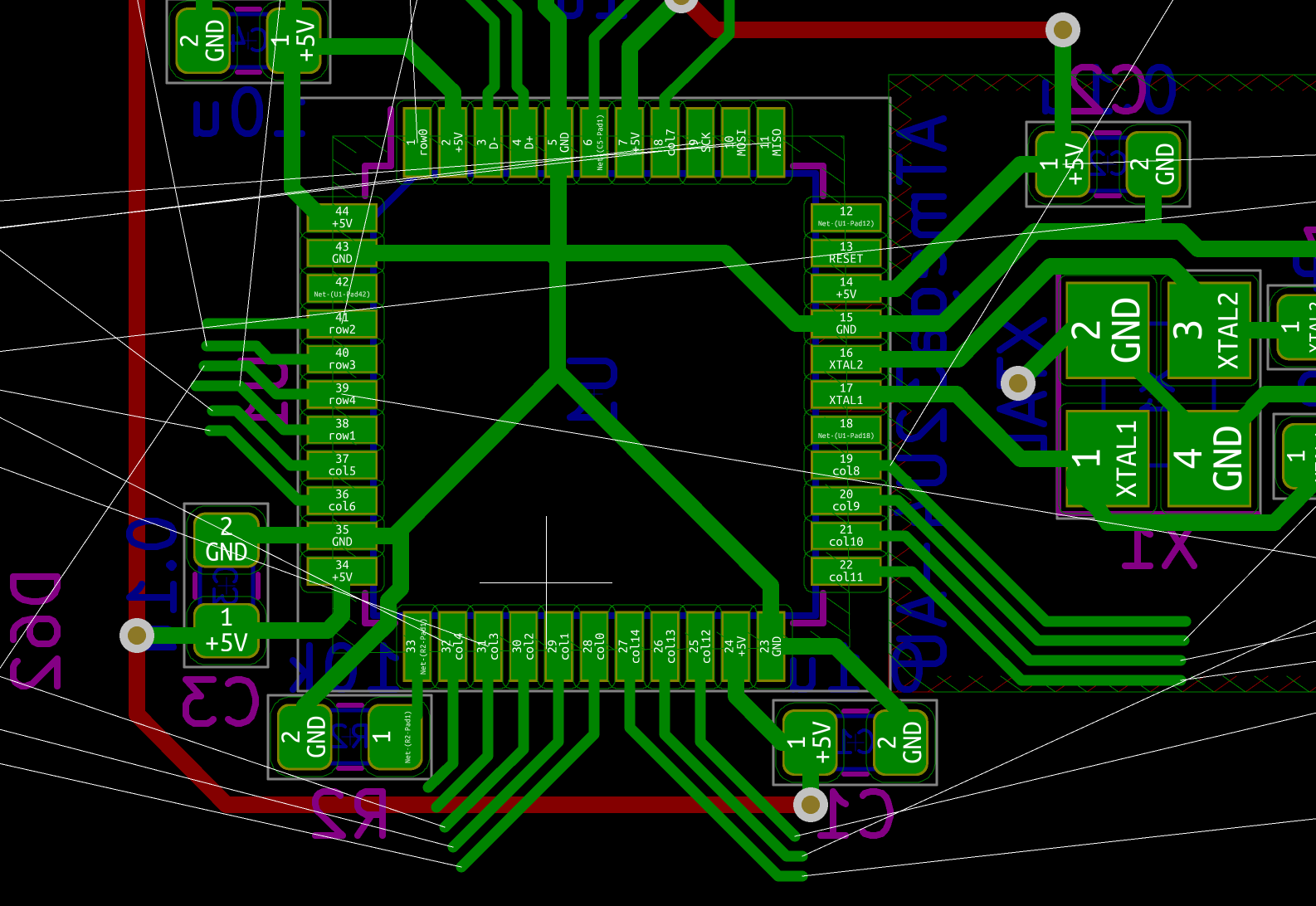
While doing that, it appears that there is a small issue on the left part of the MCU. row4 has been placed right between row1 and row3:
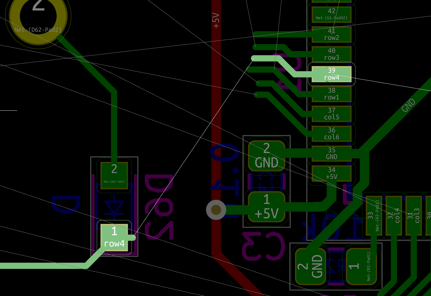
Ideally, row4 should be on the MCU pad 38 because it is to be connected directly at the bottom, while row1 and the other rows have to be connected on the left or middle part of the PCB.
Going back to the schema, it is easy to swap row4 and row1:
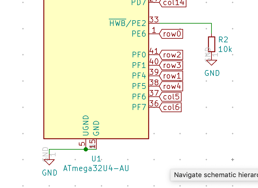
Routing again a bit more the left rows and columns, and it looks like it’s not yet perfect. There’s a conflict between col5, col6 and row4:
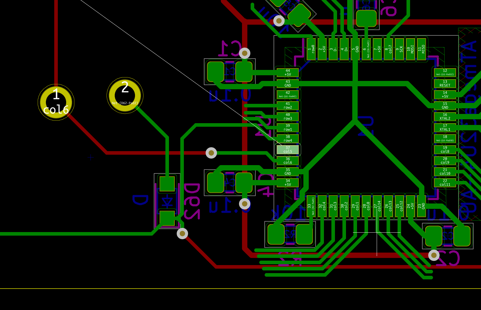
It seems much more natural to have row4 at the bottom on pad 36, then col5 and col6 (from the bottom to up), this prevents crossing those three tracks:
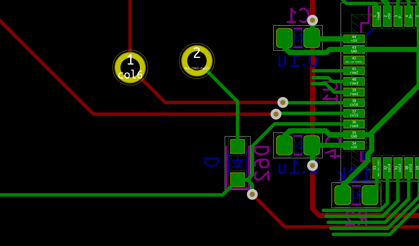
To connect the left columns (from col1 to col5), the more appealing way to do that is to group the traces as a kind of bus that connects to a pad on the last column row. Since the columns are connected on the F.Cu layer, it makes sense to convert the B.Cu traces out of the MCU with vias:
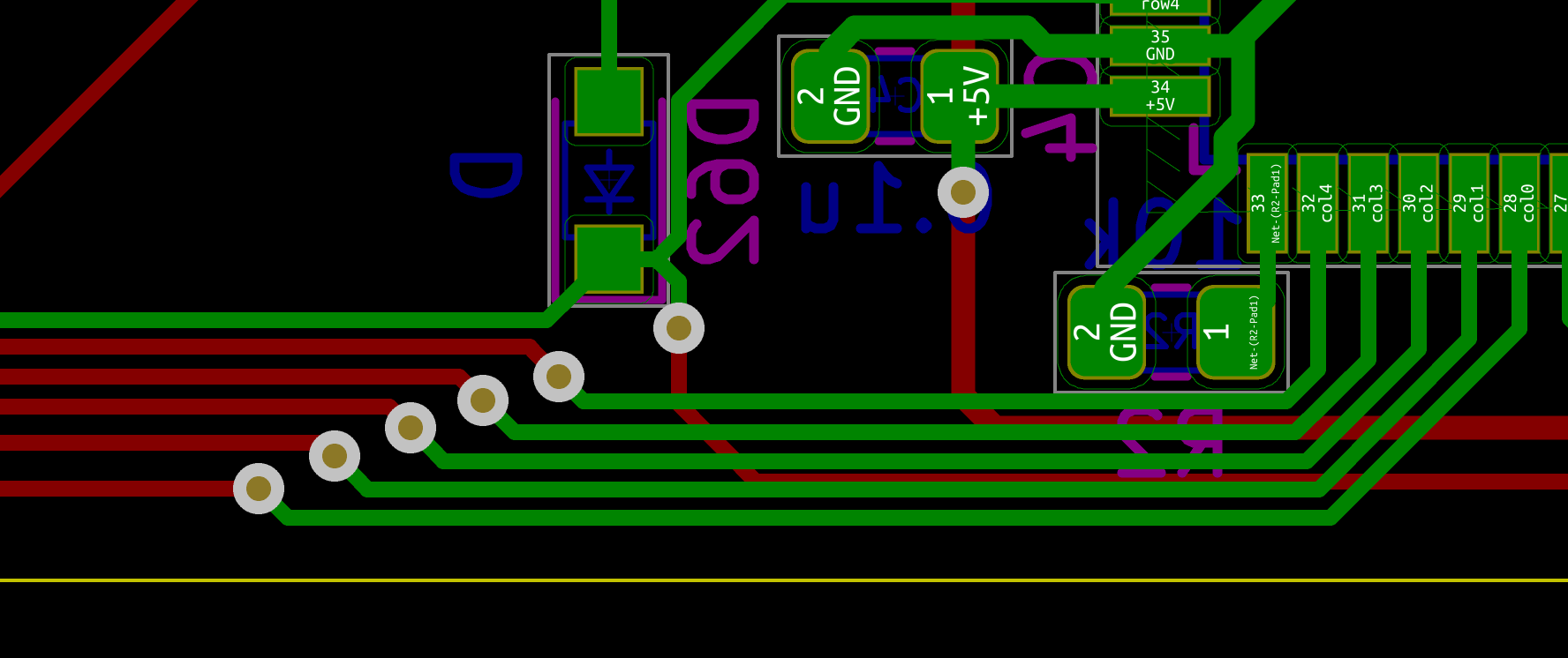
If all the traces follows the same model, it can be made visually appealing:
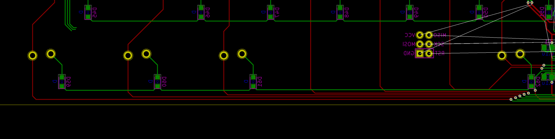
Now let’s hook the right columns (col8 to col14). Once again the idea is to group the traces together, first on B.Cu then switch to F.Cu to be able to cross the B.Cu row4:
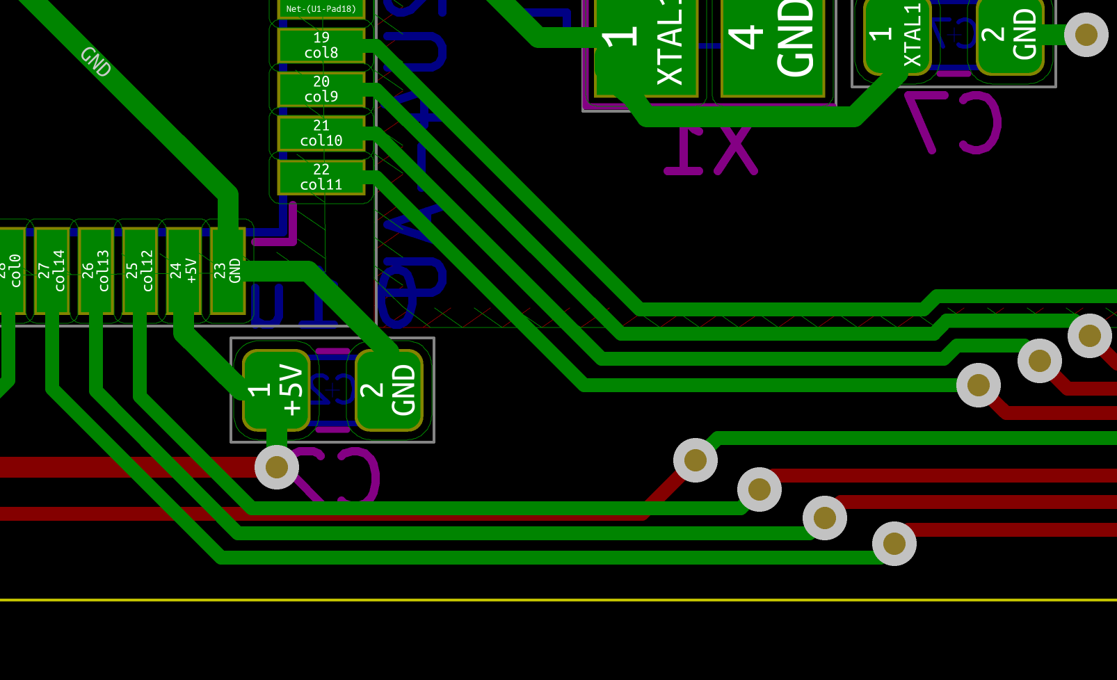
While doing that, make sure to not route the tracks too close to the border (or check the manufacturer clearance first). Then, keep tracing all tracks to their respective columns with the same kind of layout:
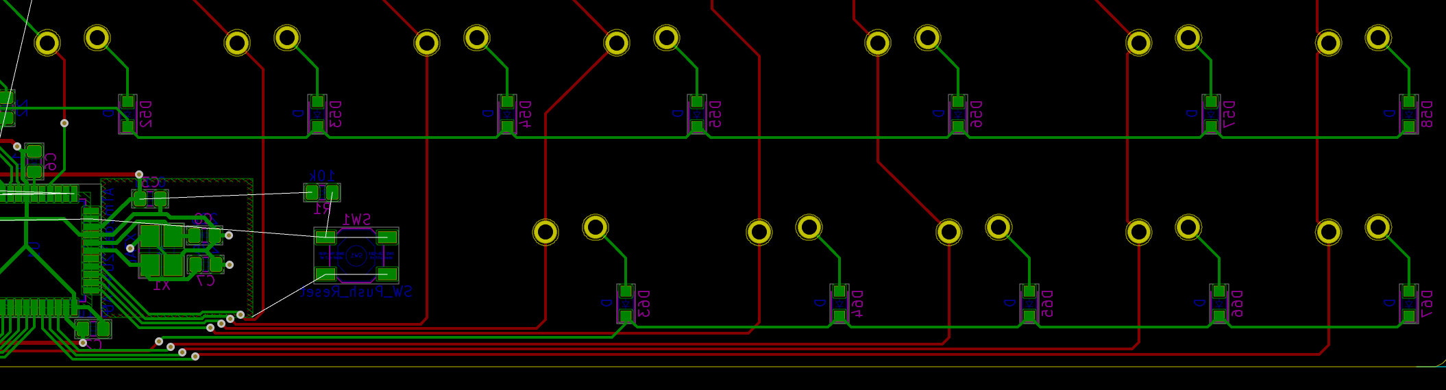
And finally, the last part of the matrix to be connected are the remaining rows (from row0 to row3, as row4 is already connected). There are multiple solutions (in fact any column in-between would work). But once again, I’m afraid I’ll have to rearrange the MCU pads:
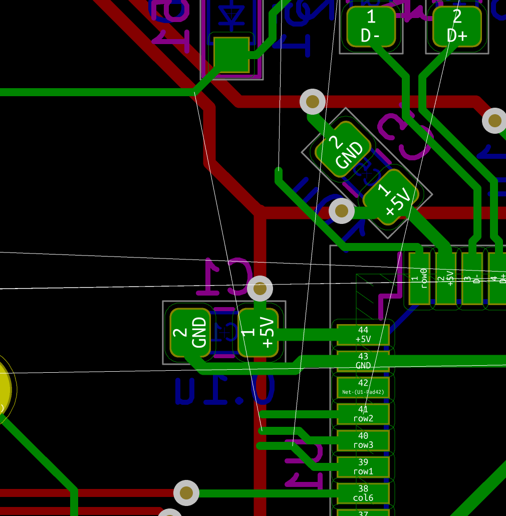
There’s row3 at a very short distance from pad 1, so it makes sense to connect it there. I’m going to connect the rows from the left part and down between row3 and row4 as this will minimize the number of crossings:
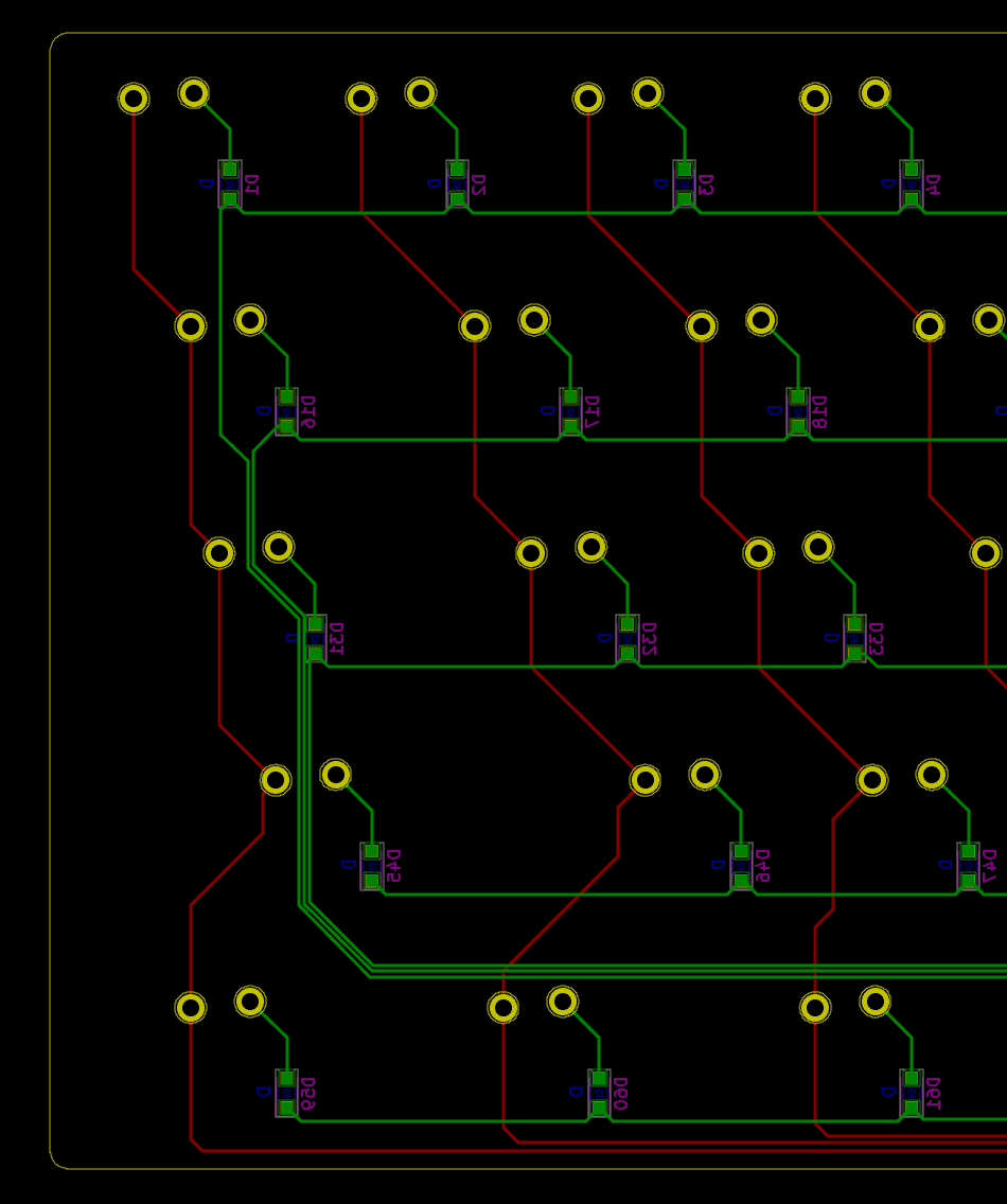
But then arriving to the MCU it’s clearly not in the right order:
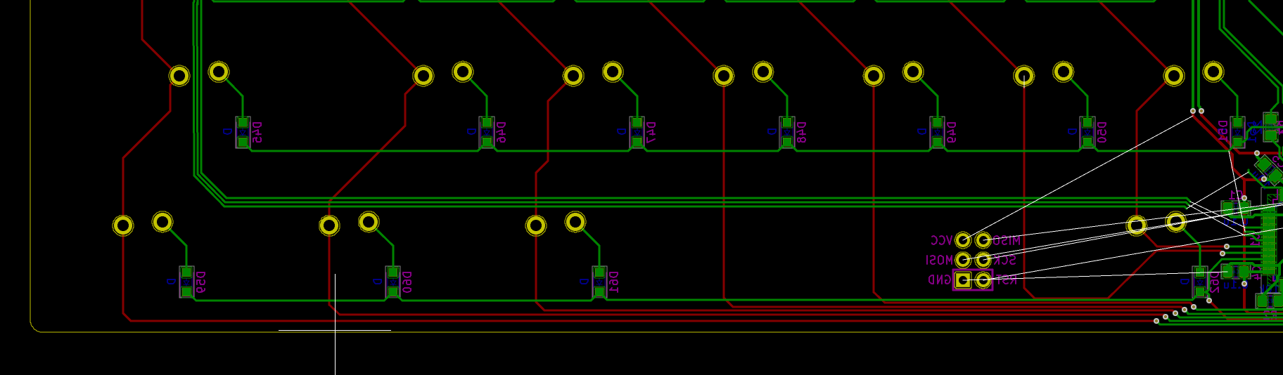
Let’s rearrange the rows in top down order in the schematic:
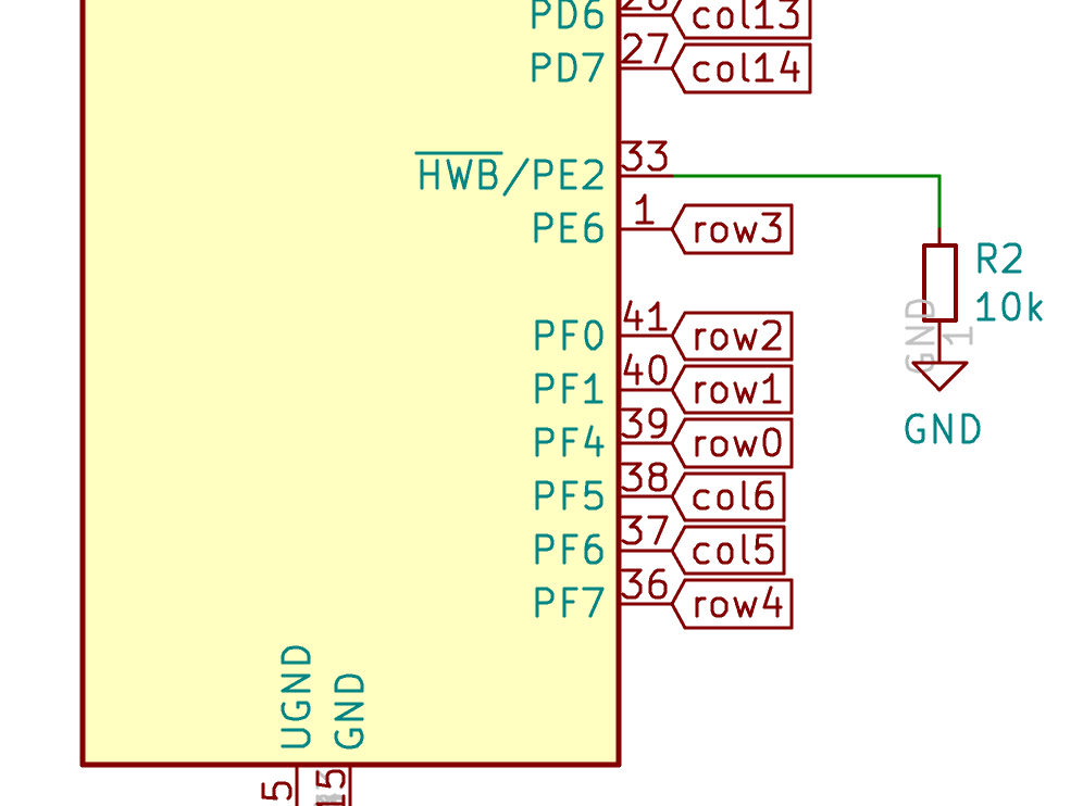
And after updating the PCB from the schematic, I can finally connect the remaining rows:
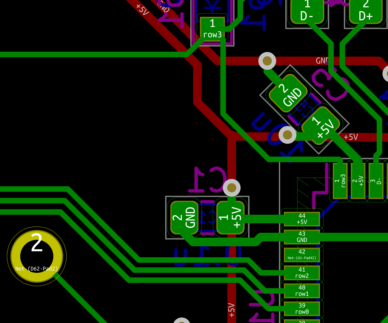
I still need to connect the reset button and the ISP header. Once everything has been done, it’s just a matter of finding its natural location (close to their assigned pads) and orientation (to minimize tracks crossings):
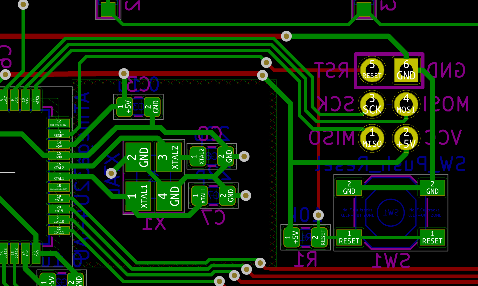
I had to divert col8 around the reset button and ISP header because it was too much in the way, but in the end it was possible to connect those components without too many vias.
Before going any further, I need to check the routing is correct. It’s easy to forget a connection or to cross two traces without noticing. Hopefully, Kicad has the Design Rules Checker feature which allows to check all those mistakes, but also the manufacturer clearances.
It can give the following errors:
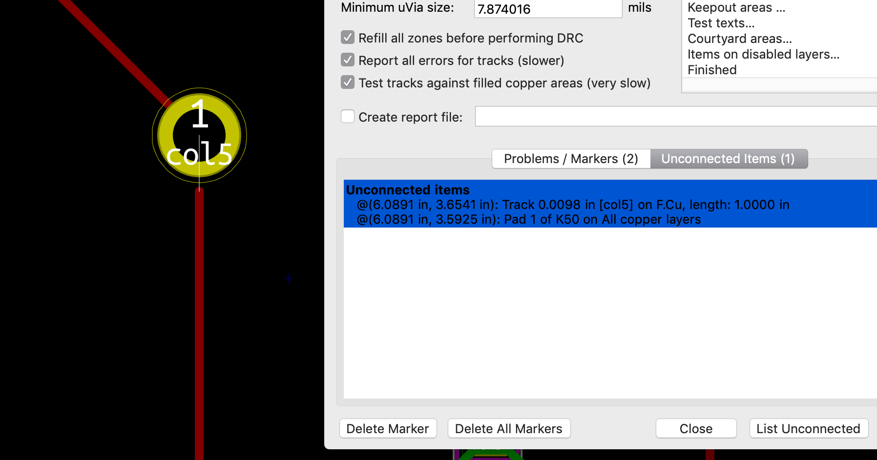
Thankfully this one is easy to fix.
When looking at the 3D rendering of the PCB, you can notice the following issues:
Let’s edit the footprints to remove the solder-mask on the top layer pads, but also display the switch value at least on the back.
Open the footprint editor, locate the Alps-1U footprint and select the left pad:
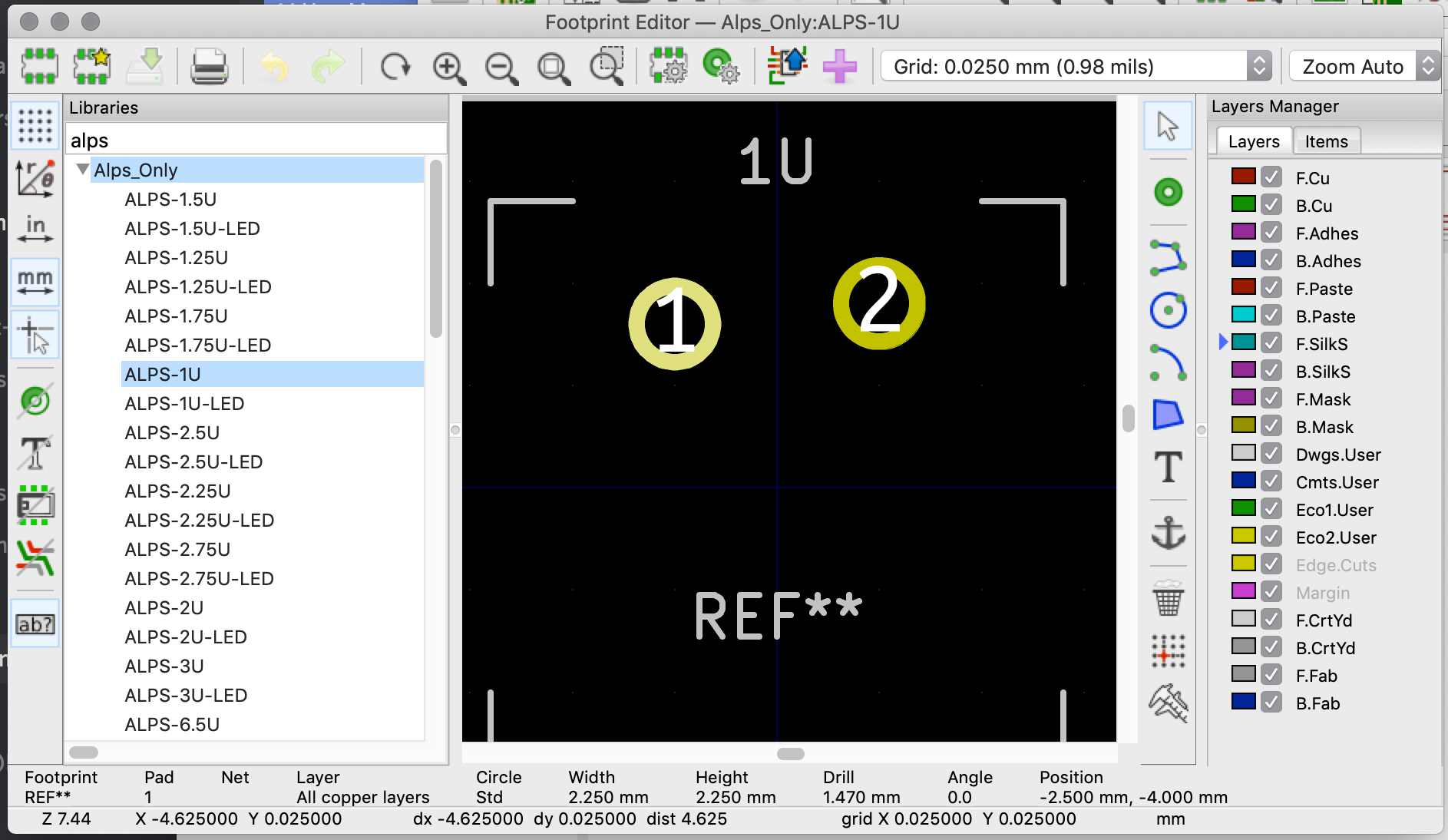
Edit the pad properties (e shortcut), and make sure that both F.Mask and B.Mask are checked:
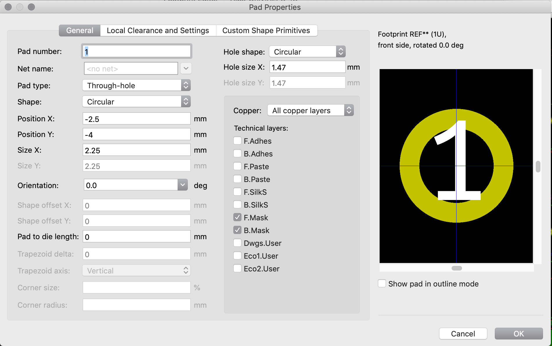
Do the same for the second pad. Then place a new text near the top of the footprint enter %V in the Text entry box (that will reflect the component value, which happens for our switch to be the key name or symbol), chose the B.SilkS layer and check the mirrored checkbox:

If you also want the key name to be displayed on the front, add another text but chose the F.SilkS layer and unselect the mirrored checkbox.
Save the footprint, then do the same for the other footprint sizes.
Once done, the PCB needs to be updated. In the PCB editor, select the Tools → Update Footprints from Library. In the dialog box, select all components with reference K??, check the three checkboxes so that all the text components will be updated and press update:
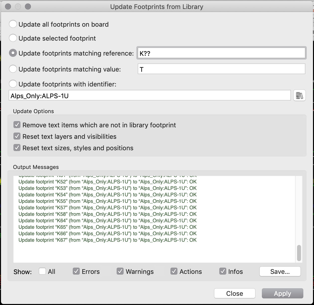
Check the 3D Viewer to see the rendered silkscreen on the front and back:
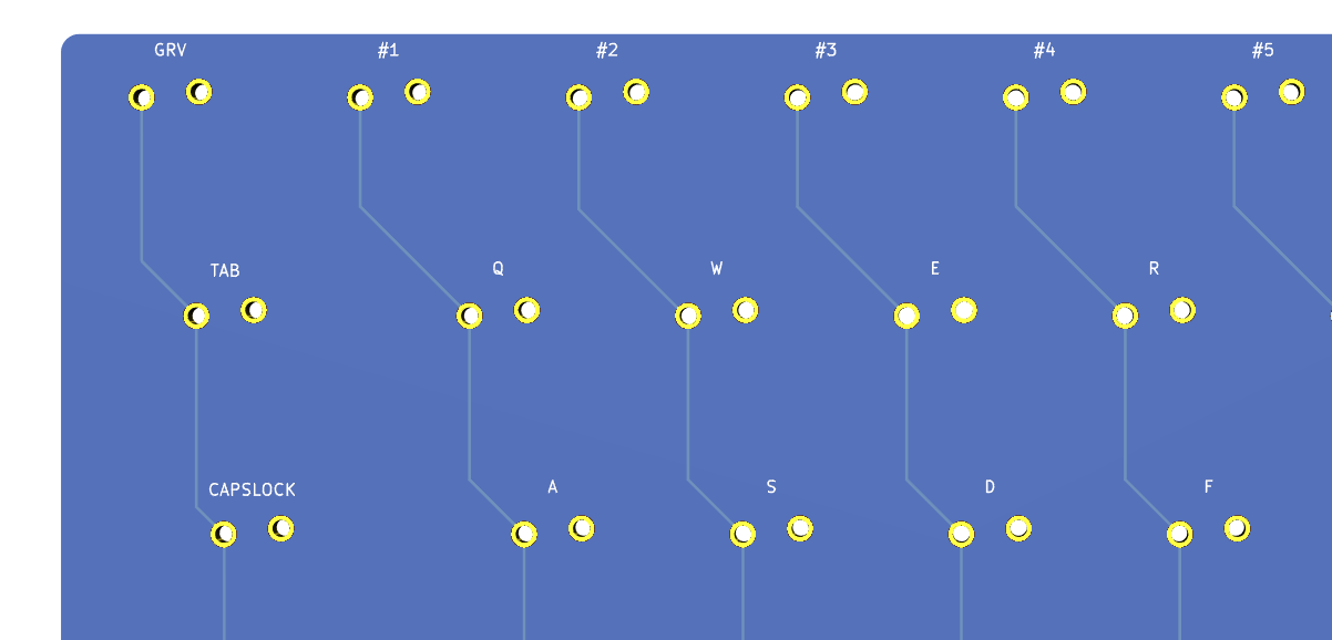
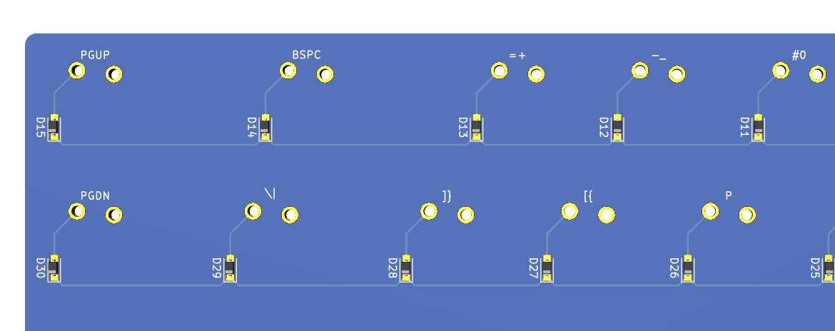
Unfortunately, we did this in the ai03 library so the modification can’t be committed to our PCB repository, because this library was added as a git submodule. Hopefully, I did the modifications in a fork of ai03 library (sorry, only Alps, no MX), so instead of adding ai03 submodule, you can add mine: git@github.com:masterzen/MX_Alps_Hybrid.git. And if you followed this article from the beginning, you can update the submodule with mine (see the How to change git submodule remote).
But wouldn’t it be a really cool PCB without at least a few silkscreen art?
The idea is to draw a vector logo (for instance in Adobe Illustrator or Inkscape), then import it as a footprint in Kicad.
Since this is an Alps based board, I thought it would be nice to have a mountain silhouette as the logo. Because I’m unable to create such art by myself, I downloaded a nice mountain wireframe in SVG from the Creative Commons Clipart website, loaded it in Inkscape and added the keyboard name (I had to rework the SVG to fix a few issues from there to there). Since this will go in the F.SilkS layer, I named the Inkscape layer F.SilkS:
![]()
If you want to add text, make sure to convert the text to paths (with the Object to path inkscape function), otherwise it won’t be imported.
Save the file into the format Inkscape SVG. Kicad doesn’t yet support importing SVG files directly, so we first have to convert the vector file to a format that Kicad can read. There are several possibilities:
I tried both method, and I won’t recommend the first one, because it is really painful to recreate all the zones in Kicad. Instead I’m going to show how to convert the SVG to a format Kicad can understand.
I wasn’t able to make the svg2shenzen Inkscape extension work correctly on my mac, so I resorted to using svg2mod which worked fine.
First install this tool with pip3 install git+https://github.com/svg2mod/svg2mod. Then run it on the svg file:
% svg2mod -i logo.svg -o ../local.pretty/logo -f 0.85 --name logo
Parsing SVG...
No handler for element {http://www.w3.org/2000/svg}defs
No handler for element {http://sodipodi.sourceforge.net/DTD/sodipodi-0.dtd}namedview
No handler for element {http://www.w3.org/2000/svg}metadata
transform: matrix [4.9686689, 0.0, 0.0, 5.4800484, -251.10361, -536.90405]
transform: matrix [0.05325035, 0.0, 0.0, 0.0482812, 50.5374, 97.974326]
transform: matrix [0.05325035, 0.0, 0.0, 0.0482812, 50.5374, 97.974326]
transform: matrix [0.05325035, 0.0, 0.0, 0.0482812, 50.5374, 97.974326]
transform: matrix [0.05325035, 0.0, 0.0, 0.0482812, 50.5374, 97.974326]
transform: matrix [4.9451996, 0.0, 0.0, 6.2660263, 266.42682, -668.87041]
Found SVG layer: F.SilkS
Writing module file: ../local.pretty/logo.kicad_mod
    Writing polygon with 5 points
    Writing polygon with 7 points
    Writing polygon with 22 points
    Writing polygon with 161 points
    Inlining 1 segments...
      Found insertion point: 0, 6
    Writing polygon with 22 points
    Writing polygon with 21 points
    Writing polygon with 28 points
    Inlining 1 segments...
      Found insertion point: 0, 0
    Writing polygon with 84 points
    Writing polygon with 31 points
This produces a Kicad footprint, which we can view in the footprint editor:
![]()
Note that I created it in the local library I used earlier to be able to commit it in my repository.
Next, place this footprint (o shortcut) on the PCB:
![]()
Unfortunately it isn’t possible to resize a footprint. The only way to resize such footprint is to regenerate it with a different resizing factor in svg2mod (the -f argument in the command above). This requires a few trials before finding the correct factor.
Let’s also do a small back-side logo. With the exact same logo, it is possible to flip it in Inkscape, rename the layer to B.SilkS, and finally save the SVG to another file. When converting the small logo to a Kicad footprint, make sure to use a very small -f factor (0.15 exactly). I can then place it on the PCB:
![]()
Finally, I’ve also added a small copyright and version number text on the B.SilkS layer.
Here’s the result so far:
![]()
And the back:
![]()
I’ve seen a lot of 2-layers keyboard PCB design that use ground fills on both faces (not that the ai03 tutorial is not doing this). I believe the attempt here is to implement some kind of EMI reduction or crosstalk reduction. I tend to think it might be counterproductive to have such ground fills (or pour). First those won’t reduce EMI, only proper bypass/decoupling capacitors, conscious routing of high frequency trace (to minimize loops area), or using a ground grid scheme can help reduce EMI on 2 layers board (and on 4+ layers boards, using uninterrupted ground/power planes). Some will say that it helps for heat dissipation, or that they are forced to use ground fills for manufacturing reasons or that they paid for the copper, so better use all of it. Those might be valid reasons, but for such project a ground fill might really be overkill.
Don’t get me wrong, on a multilayer PCB, having uninterrupted ground planes is essential to reduce EMI. But on 2-layers PCB, it will be hard to have an uninterrupted ground (hence we talk about ground fill, not plane). Any slot in the ground fill that would interrupt a return current will just become an antenna. A ground fill might reduce cross-talks between traces, but it might also act as an antenna if it’s too thin and long. So if you want to add a ground fill, just make sure you take this into account.
That’s the reason we routed GND as a trace earlier, at least there’s an uninterrupted return path for the current. We could stop the design here and produce the board as is, it would definitely work.
Still for the exercise, I’m going to try to add a ground fill on both faces, but doing so correctly (or at least trying).
Let’s see how we can add a ground pour. In kicad use the Add Filled Zone tool and draw a large rectangle in the B.Cu layer around the whole PCB. To ease drawing, it’s better to use a 20 mils grid settings:

Keep going around the board:
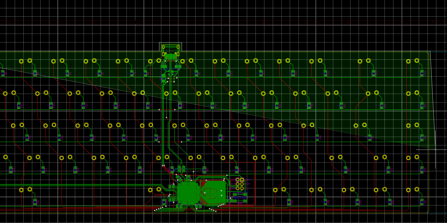
And connect back to the starting point. This gives this:
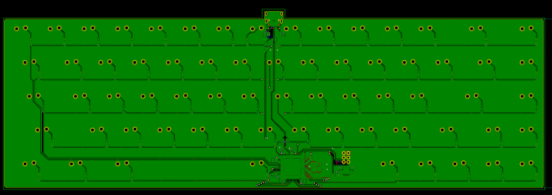
This is far from being perfect, because it merged the crystal oscillator ground island we designed earlier. I have to add a keep out zone to disconnect the island. This can be done by right-clicking on the ground zone and choose Zones → Add a Zone Cutout, then draw a rectangle around the crystal oscillator ground zone, spaced by 20 mil:
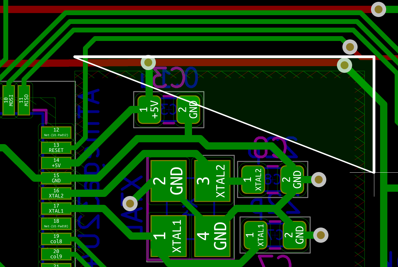
Next, let’s duplicate the same copper fill on the other side by going again in the zone contextual menu and choosing Duplicate Zone onto layer and chose GND on F.Cu:
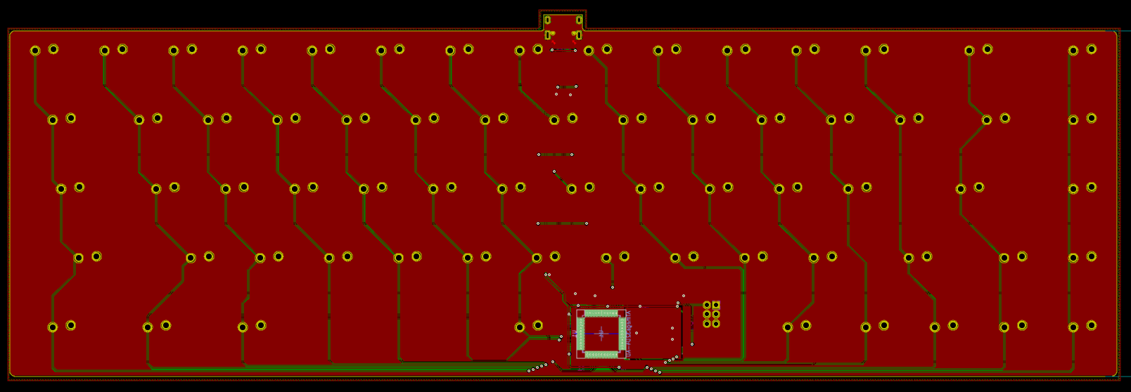
Note that when creating a zone, make sure to select the Pad connection thermal relief option. A set of clearance parameters that works fine is 6 mils for the regular clearance, 10 mils of minimum width and 20 mils for both thermal clearances. The thermal clearance and pad connection are very important settings, without those, hand-soldering the PCB might be difficult as the ground fill copper would dissipate the soldering iron heat and the solder wouldn’t flow correctly. If the PCB is to be assembled at a factory then it wouldn’t be an issue.
Let’s look what we can do to make the copper fill better. First we have to make sure the copper fills are properly grounded together (they need to have the same potential to not be a gigantic antenna) by stitching vias from there to there. This will reduce the plane capacitance, but that’s not an issue since we have plenty of decoupling capacitors around the MCU. The idea is to reduce the potentiality of any part becoming an antenna. Place a few vias from there to there or use the Via Stitching kicad plugin to do that. Here’s an example with the Via Stitching plugin with a grid of 32 mm (it’s possible to add more vias, but there’s no need to make a Swiss cheese):
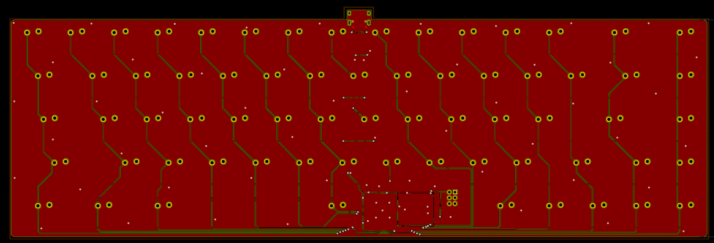
It’s not finished yet. If the return current of the D+/D- goes into the F.Cu ground fill back to the USB connector, the path of least impedance (that’s the path of high frequency signals) would cross several horizontal traces. This isn’t good, the current loop area will be large (those return currents will have to turn around the obstacles increasing the loop area). The largest the current loop, the largest the electromagnetic emissions. To circumvent this issue, we can add a few pairs of vias around those horizontal traces that split the F.Cu plane. To do that, work in Do not Show Filled Zone mode and create small GND tracks and vias across the horizontal lines:
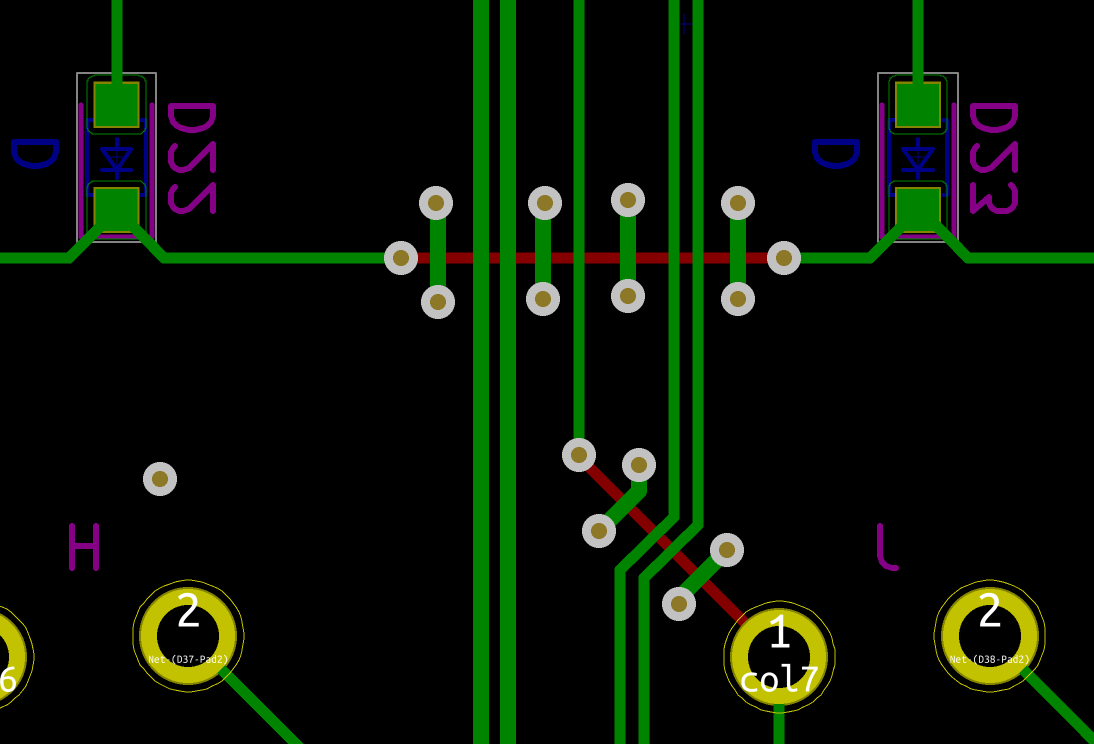
Going back to the visible Filled Zone mode, this would look like this:
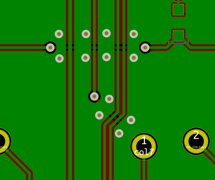
Next, repeat that around all the zone splits that the differential pair crosses:
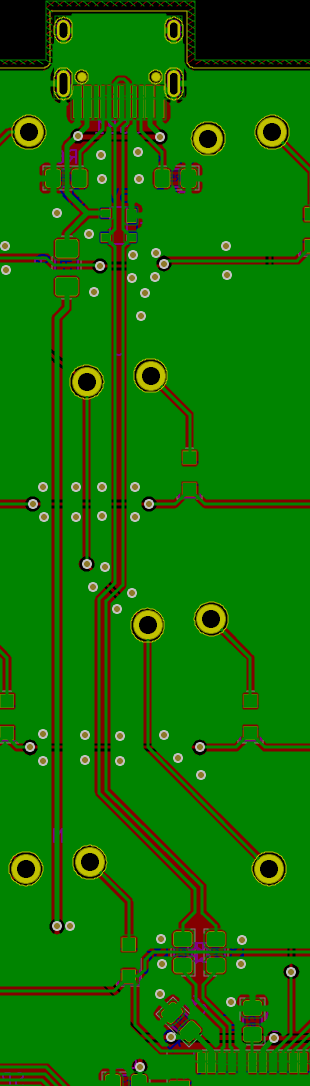 ](/images/uploads/2020/05/pcb-route-all-vias-bridges.png)
In this series first part, I opted for an USB schema where I connected the shield and ground.
There are endless debates on the Internet about whether it’s correct or not to connect shield and ground. I did a lot of research, because I had the feeling that it might be wrong.
The USB cable shield is there to prevent electromagnetic outside noise from coupling with the USB data wires, but also to protect the outside world from noise that could be generated by the USB data wires. Additionally, the USB port shield can be susceptible to electrostatic discharge through the USB connector.
What makes the matter complex is that the USB norm doesn’t tell exactly what should be done. In fact, it depends on a number of factors, among them: is it the host or device? Is it bus powered? self powered? powered by mains? etc.
If we focus on this project, I’m building a keyboard PCB (so from an USB standpoint a device powered through the bus), which I plan to enclose in an aluminium case.
This PCB will be connected to a computer (what’s the point if not?), and thus the device signal ground will be the same as the host signal ground and the cable shield will be connected to the host shield. On desktop computers the host shield is usually connected to earth ground. On laptops, it really depends. Anyway, let’s assume that the host shield is somehow correct.
Connecting the USB signal ground GND to the USB port shield will have the drawback of possibly having a return current using the cable shield, negating the effect of the shield (the shield would possibly induce noise in the USB data lines). It would also mean that potentially the keyboard case would be also connected to the USB singal ground, which wouldn’t be great in case of an electrostatic discharge: a tension could then be seen on ground (the PRTR5V0U2X ESD protection device we use can protect VCC but not GND).
Ideally the USB port shield should be connected to the metallic case (by using an EMI gasket, a direct connection or through metalized holes and screws in the PCB). That’s one of the reasons more and more custom keyboards are using the Unified USB Daughterboard. When the USB port shield is connected to the case, this one protects the PCB from EMI (and also helps reduce EMI coming from the PCB), but it also contains any ESD and direct them to the host.
So, would the shield be fully disconnected from the USB GND? In fact, no that would be worst. In case of an ESD, an electrical arc could form between the case and any close traces of the PCB (well after the ESD protection device) risking damaging the components (because the surge wouldn’t go through anything that would prevent it).
After researching literature for a while (especially Henry W. Ott’s EMC book), I concluded that a good plan would be to redesign the electric schema of the USB shield, and this part of the PCB. The aim is to create a dedicated I/O ground plane under the USB port shield that would be connected to the PCB GND through a ferrite bead. The other option could be to use a RC filter built of a 1MOhm resistor and a 4.7nF capacitor. But there’s not a lot of room on the PCB at this place so the ferrite bead is a good option.
A ferrite bead is a small common choke component that exists in SMD form-factor. It acts as a kind of lowpass filter. This aim is to filter out the high frequency noise that could be coupled in the shield before it can reach the USB GND or couples to the data lines. Unlike what is somewhat thought it can also help reduce the effect of an ESD. ESD spectral density is roughly around 100-500 MHz. This frequency range is specifically filtered by ferrite beads (if you wonder why, it’s because the ESD high rise time generates high frequency harmonics).
I just added a new component a Ferrite_Bead_Small with an Inductor_SMD:L_0805_2012Metric_Pad1.15x1.40mm_HandSolder footprint:
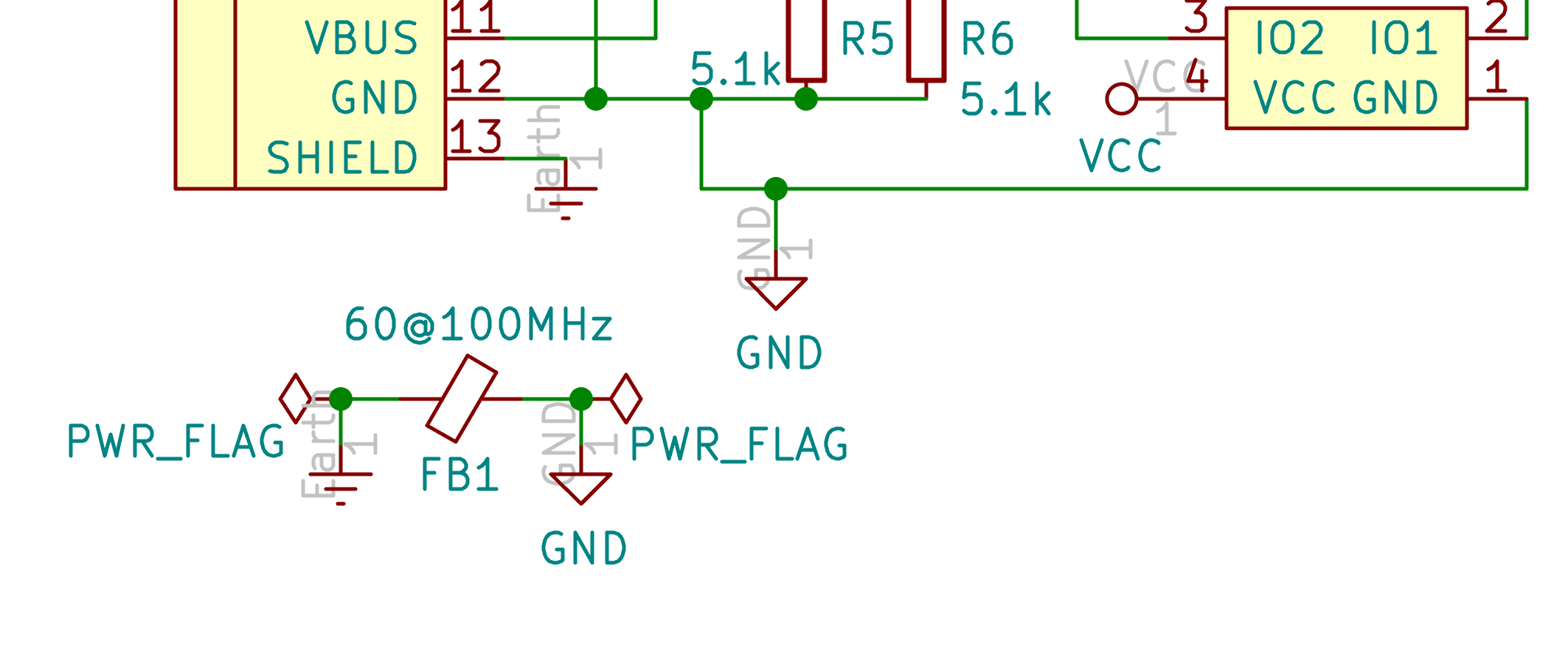
Then after annotating the schema (without annotating everything again to not change all the references), and updating the PCB, the split I/O ground fill has to be created. This can be done by first resizing the GND ground plane like this:
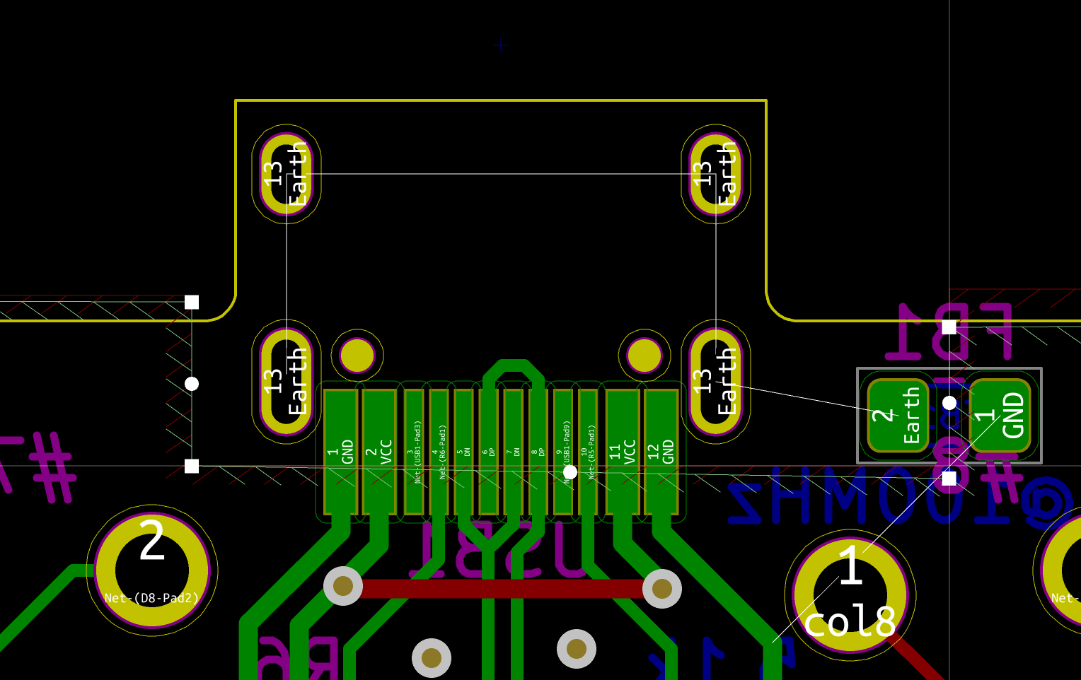
Then I can place the ferrite bead footprint across the seam between the I/O ground plane and the GND plane. Next, I can create the new I/O plane:
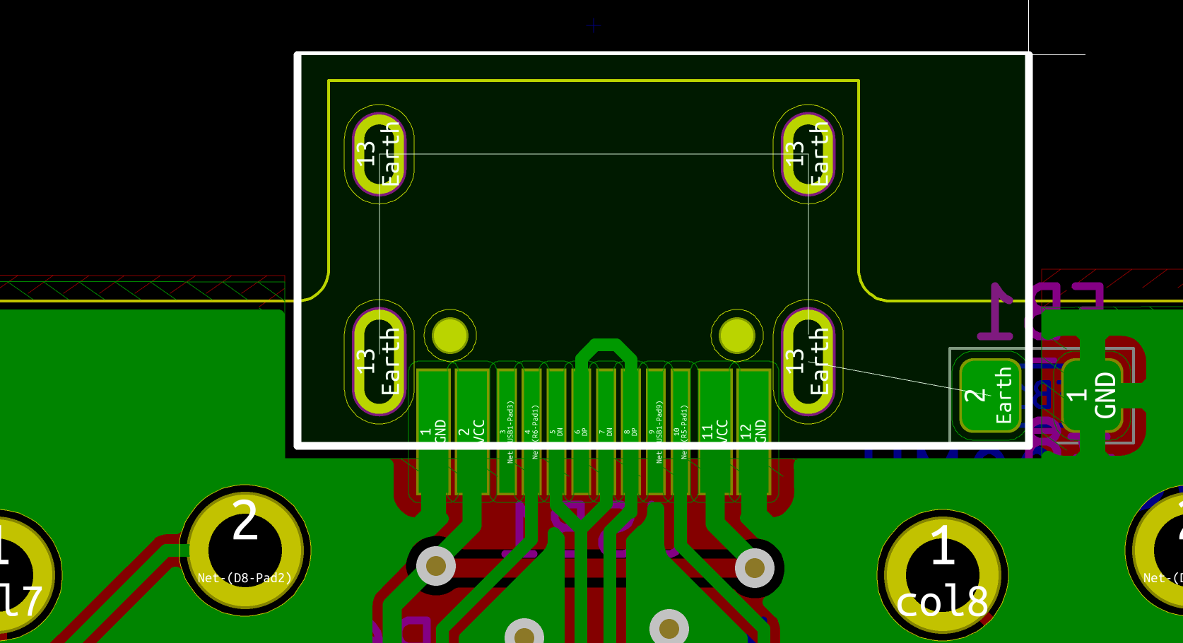
To ease creating the seam, use a coarse grid (for instance 10 mils). Finally, duplicate the zone on the F.Cu layer:
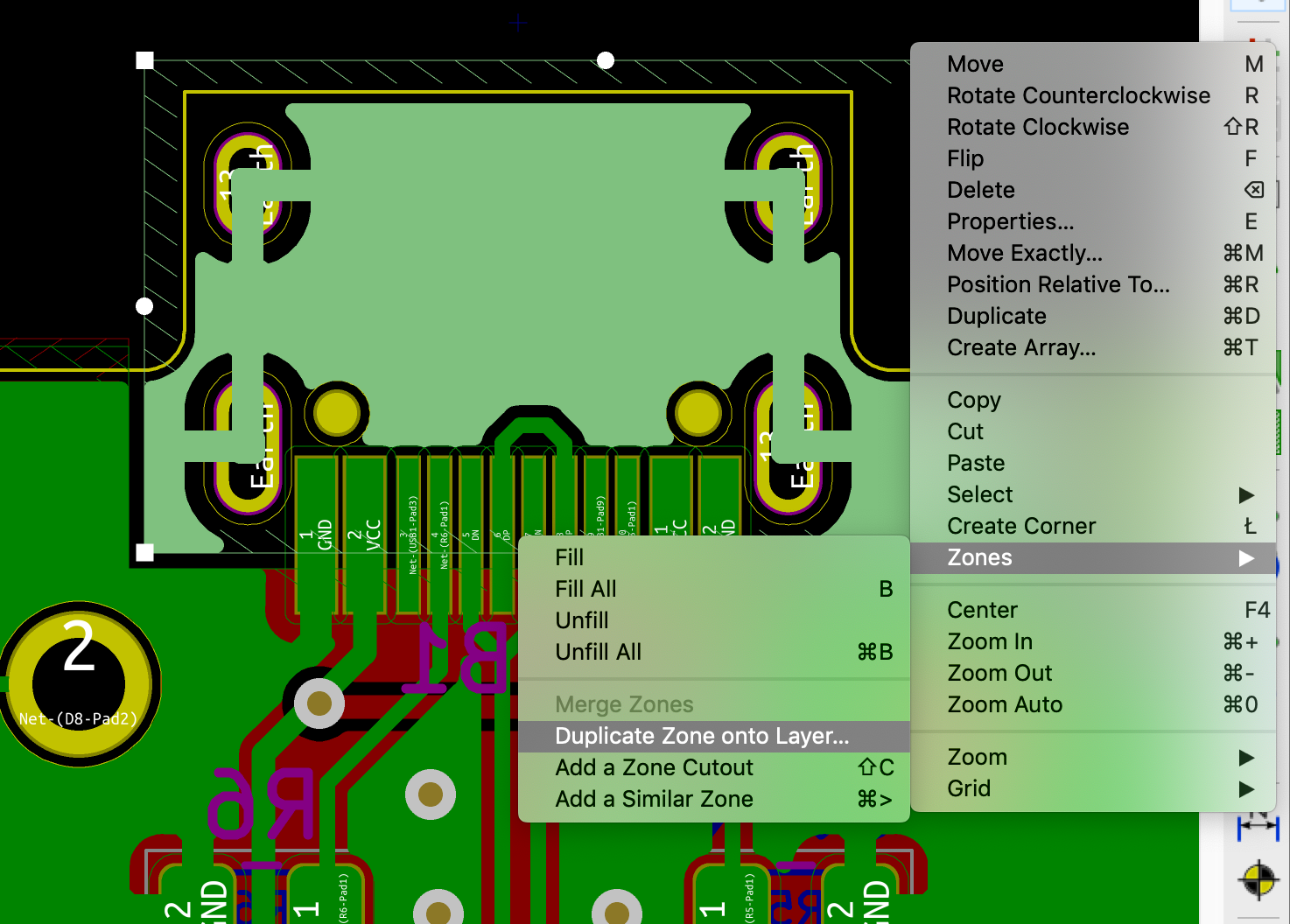
And finally, we need to make sure both planes are connected together (they are through the USB receptacle shield) by adding a few vias:
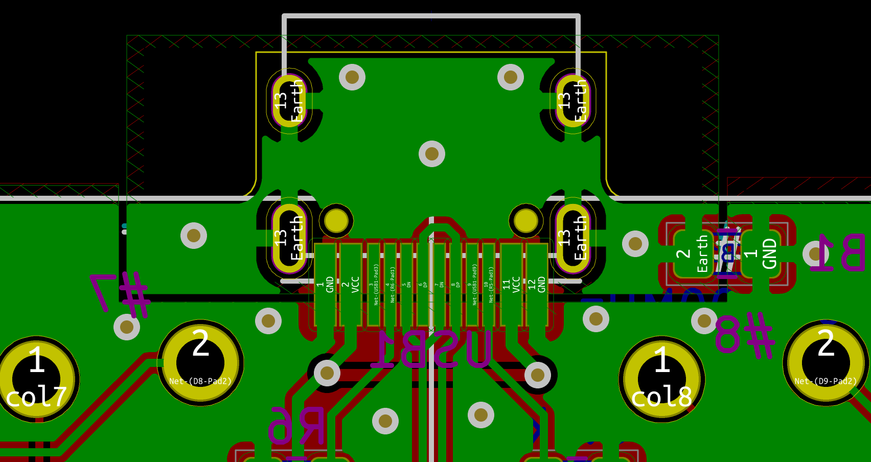
I also made the I/O zone symmetrical, to make it nicer.
Here’s the final PCB render:

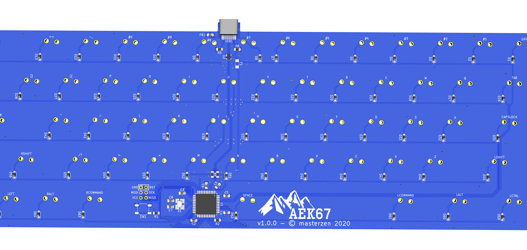
I quite like the result!
That’s all for today (it took so long to write this). In the next episode I’ll try to cover:
Thanks for following!
Welcome for the second episode of this series of post about designing a full fledged keyboard from scratch. The first episode focused on the electronic schema of the keyboard controller. This episode will cover the following topics:
Trust me, it will be probably the most boring part of this series. I’m going to design the electronic schema of 67 switches and diodes.
Since the MCU schema is taking some space in the main sheet, I recommend creating a hierarchical sheet to place the matrix components. This can be done by pressing the s shortcut and clicking anywhere in the schema. The following window should open:
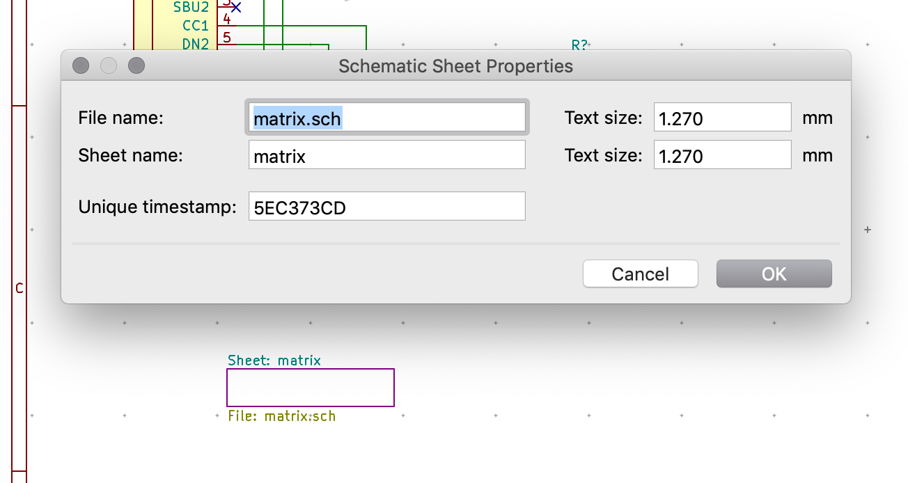
Because I’m designing the matrix, I named this new sheet matrix (yes that’s quite original).
It is possible to access this hierarchical sheet with the View → Show Hierarchical Navigator menu:
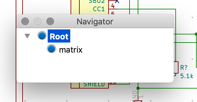
Clicking on the matrix will open this new (blank) schema sheet.
Let’s build the matrix now. As I explained in the previous article, the matrix is the combination of one switch and one diode per key. It’s cumbersome to add those components by hand for all the 67 keys, so I’m going to explain how to do it with a selection copy. There are other ways to do it, for instance by generating the schema with this tool or this other tool.
Let’s first design our key cell, by adding a SW_PUSH and a regular D diode. Next wire them as in this schema (notice that there’s no connection between the vertical and horizontal wire):
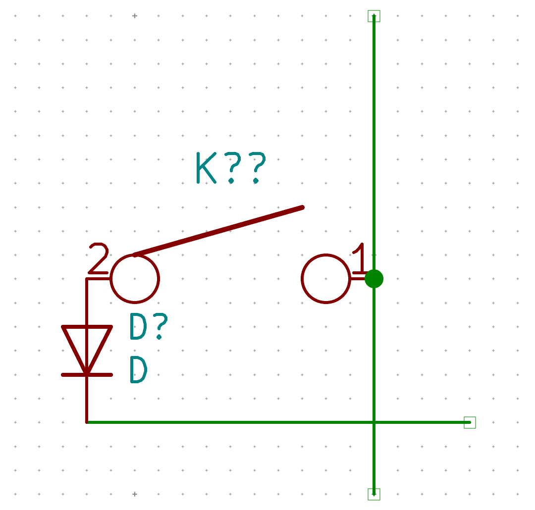
This cell forms the atomic core of the matrix. Once done (if you also are following this for your design make sure the wires have the same size as mine), maintain the shift key depressed and drag a selection around the cell (wire included). This will duplicate the selection (our cell), then move the mouse pointer so that the diode bottom pin is perfectly aligned with the first cell horizontal wire:
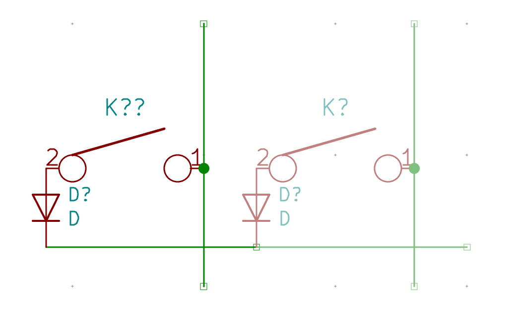
Then click the left mouse button to validate. Now repeat the shift drag selection operation on both cells at once to duplicate them and form a 4 keys schema:
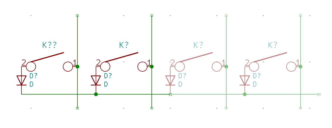
Note that it is also possible to perform the move and place with the keyboard arrow keys and enter to validate.
Next, repeat the same with the 4 cells to form a line of 8, then a line of 16 cells, and remove the last one to form a 15 keys row. If the key rows is larger than the page, you can increase the sheet size by going to File → Page Settings and change the Paper Size to A3.
This should look like this:
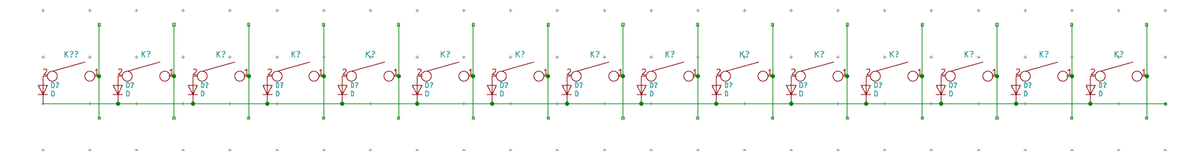
Let’s add a label to the row (Ctrl-H):
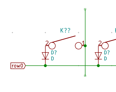
Let’s now do the other rows. I’m going to apply the same technique, just do a shift drag selection around the whole row0 and move it downward so that the wires of the columns connect:
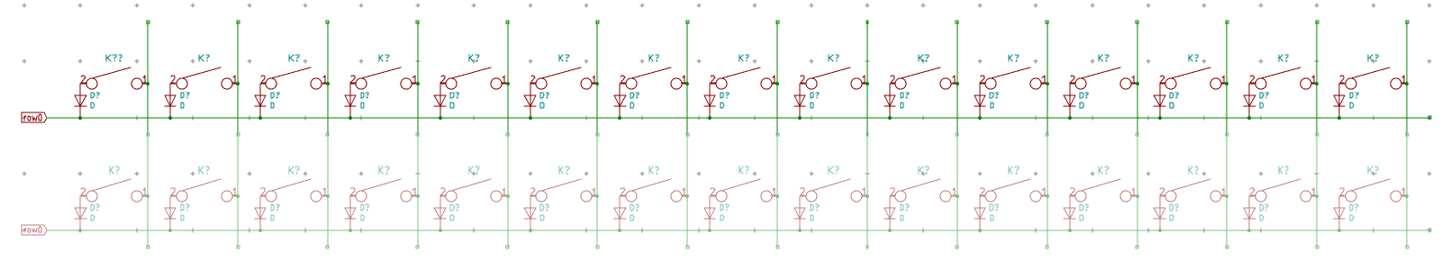
And do the same for the next 3 rows, this will give this nice array of switches:
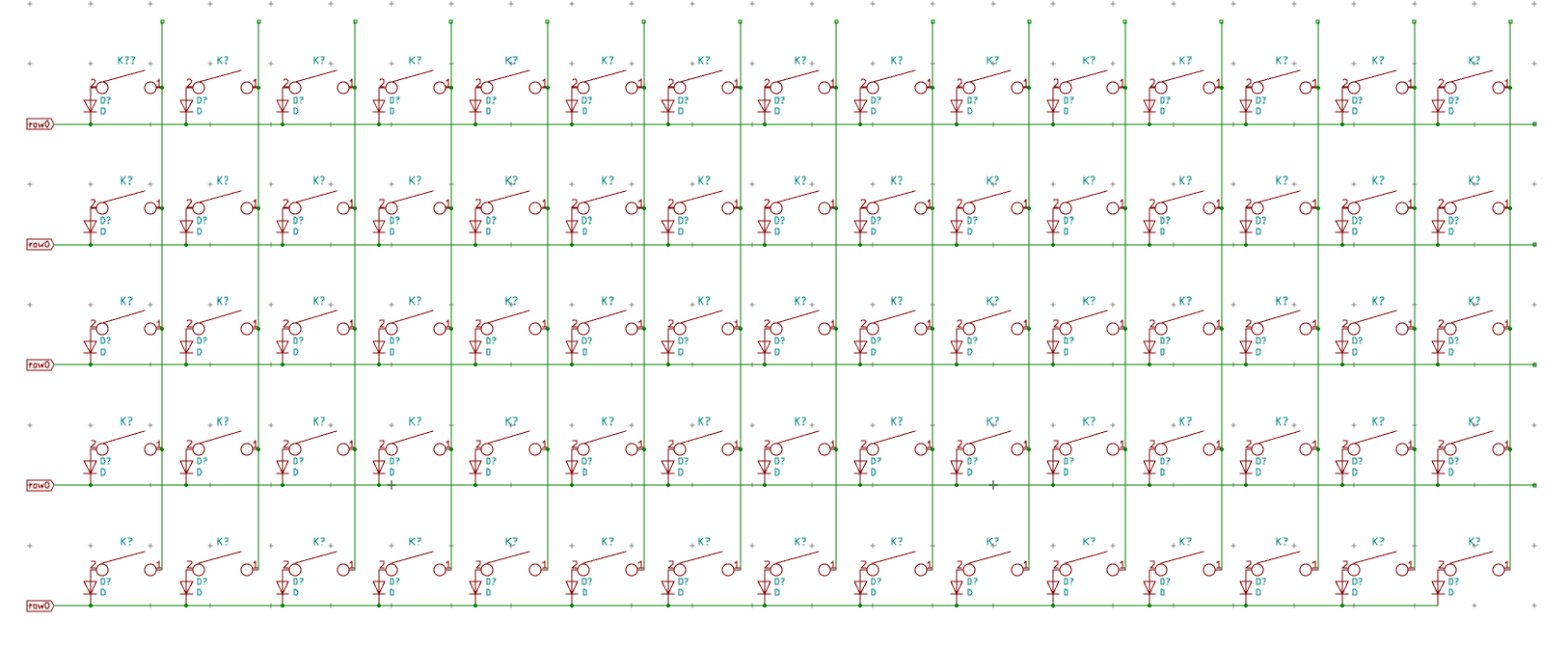
Note that I have pruned the extra vertical wires of the last row with a large regular selection and pressing the del key. It is also possible to do the same for the right extra wires on all rows.
Next, edit all the row labels to make them row1, row2, etc. The columns also needs to be labelled. Start by adding a global label on the first column and label it col0. Use the shift-select trick to create a second one, then 2 extra ones, then 4 etc until all the columns are labelled.
Edit the labels so that they are labelled from col0 to col14.
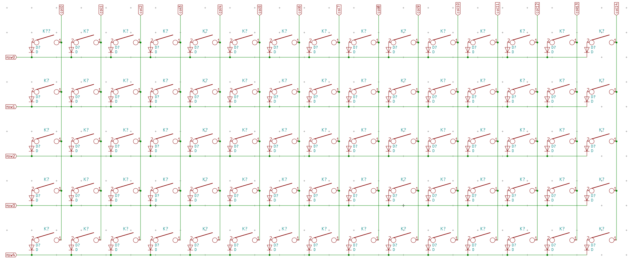
Finally that was quick! But I suspect you’ve noticed there are too many keys in this matrix. I’m going to remove some of the extraneous switches so that the wiring would look like this if laid out on the physical layout:
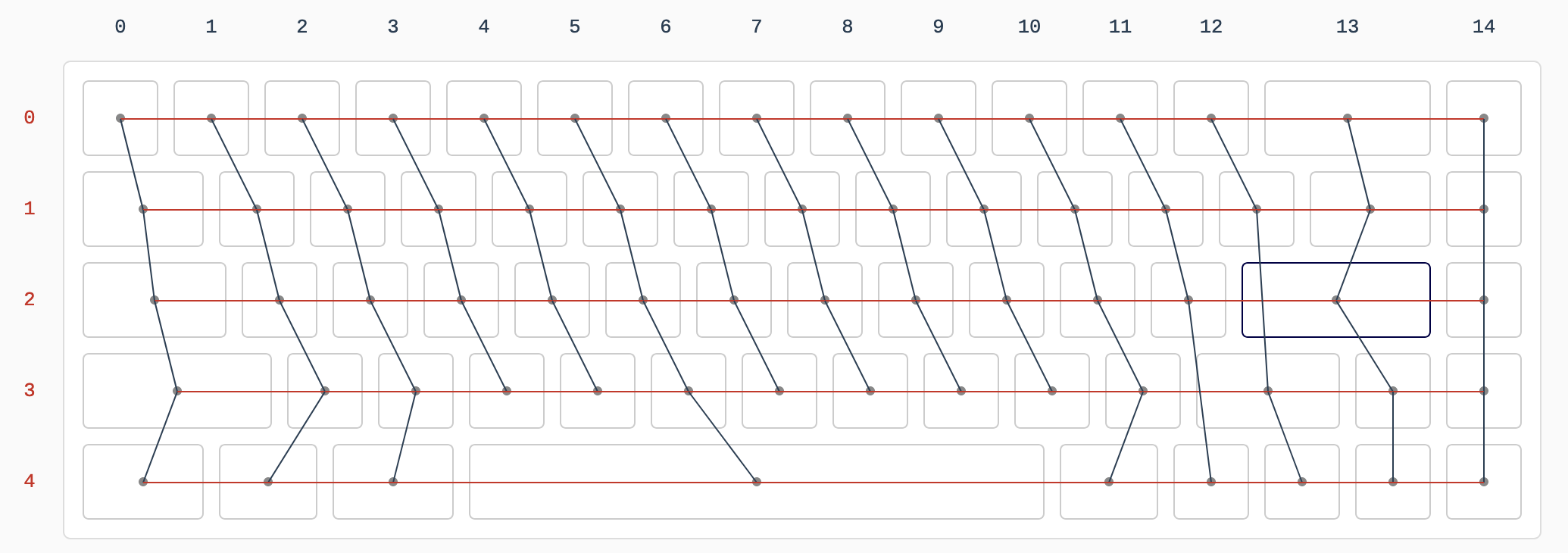
To eliminate the unneeded cells it’s as easy as selecting their switch and diode (and as less wire as possible) with a drag selection and pressing the del key.
The matrix should now look like this:
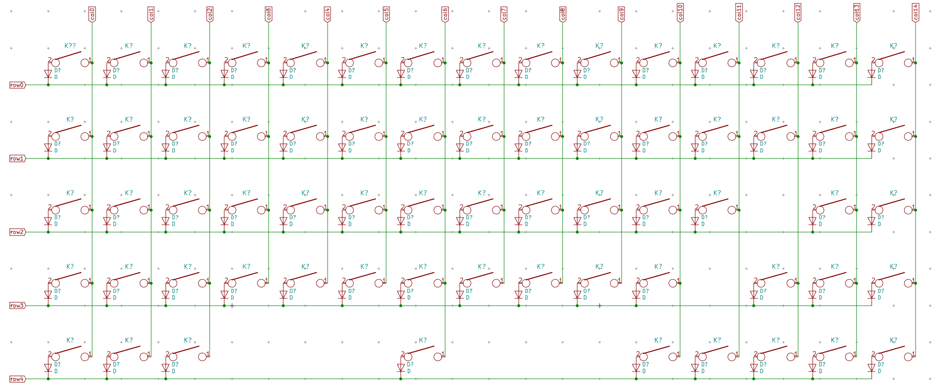
Now, I’m going to reference all the switches and diodes I just placed. Since I’m quite lazy, I’ll use the automatic referencing feature. If you want to reference switches by coordinates (ie first switch is K000, second one K001, but first of row1 is K100, etc), you’ll have to perform that manually (or write a script to directly modify the .sch file, or edit it with a text editor). I will just use increasing numbers in line.
Use the Tools → Annotate Schematics to open the annotation window:
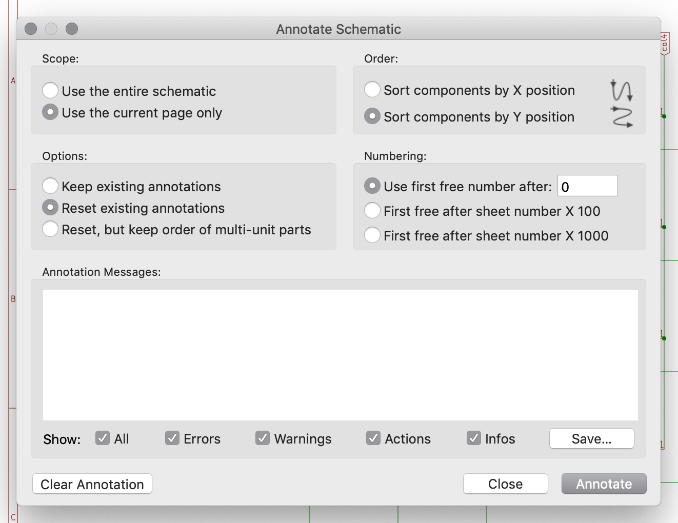
Make sure to annotate only the current page, and to Sort components by Y position. Once done, the matrix diodes and switches will have a proper unique reference identifiers. If you somehow failed, the same dialog can also erase all references (trust me, it’s easy to make a mistake, like for instance applying references to the whole schematics and not only to the current sheet).
The next step is to label each switches with their key character or name (ie K1 will be GRV, K2 #1, K17 Q, etc). This will help when laying out the PCB, because the key name will be visible, compared to referring keys only by their identifier. I could have use the key name as the identifier (for instance K_SPACE, or K_ENTER), but Kicad wants each reference to contain a number which makes things look ugly in the end.
To assign key names to the switches, I’m going to use the Tools → Edit Symbol Fields window. This opens a new dialog that allows to group components by reference or value (or both) and to edit component values all at once:
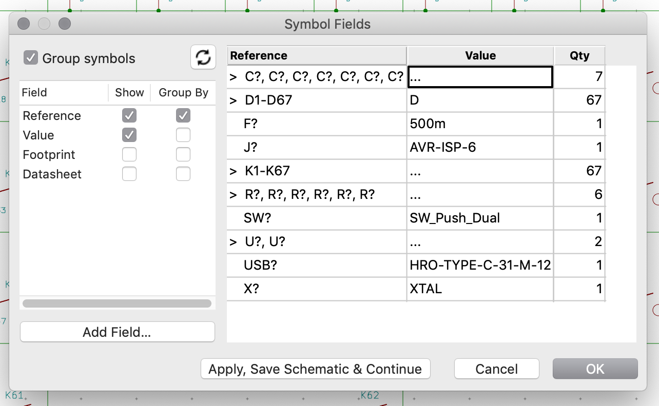
Open the K1-K67 group, and start assigning the correct key names in the value column to the switches in order:
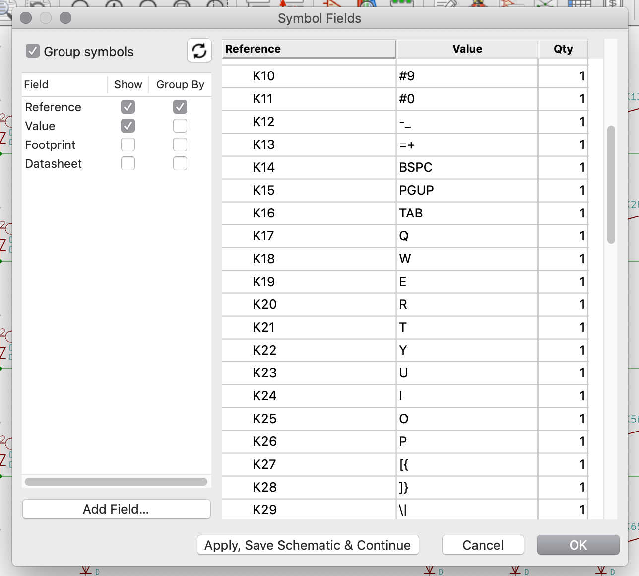
Once done, the matrix itself shouldn’t be different than it was before. The key names don’t appear, because the KEYSW symbol have the value marked as invisible. Unfortunately it isn’t possible to edit this symbol with the Symbol Editor, toggle the value visibility and reassign the symbol to all the KEYSW in the matrix. Kicad allows you to do that, but doesn’t change the visibility of the existing symbols. If I want the key name to appear I will have to edit manually all the 67 switches to turn on their value visibility or edit the matrix.sch file with a text editor. I chose to alter the matrix.sch file with the sed command. Make sure to save the schema, close it and git commit the file and project before doing this:
sed -i -r -e 's/^F 1 "([^ ]+)" H ([0-9]+) ([0-9]+) ([0-9]+) 0001 C CNN/F 1 "\1" H \2 \3 \4 0000 C CNN/' matrix.sch
Reopen the root schema, then the matrix and you should see something like this:
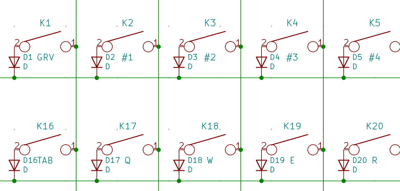
The matrix is now finished. The perfectionist among us could move the key values or diode references so that they don’t collide (but remember I’m lazy).
The next step is to finish the main schema.
Using the Tools → Annotate Symbols, I’m going to assign references to the main sheet (and only this one). Once done, to ease laying out the MCU on the PCB, I’m going to tentatively assign rows and columns to the Atmega32U4 pins.
To do that, I need to tell you a few rules about laying out our board:
D+/D- signal form a differential pair. They need to be traced as directly as possible.The physical layout of the MCU looks like this (it’s called a pinout):
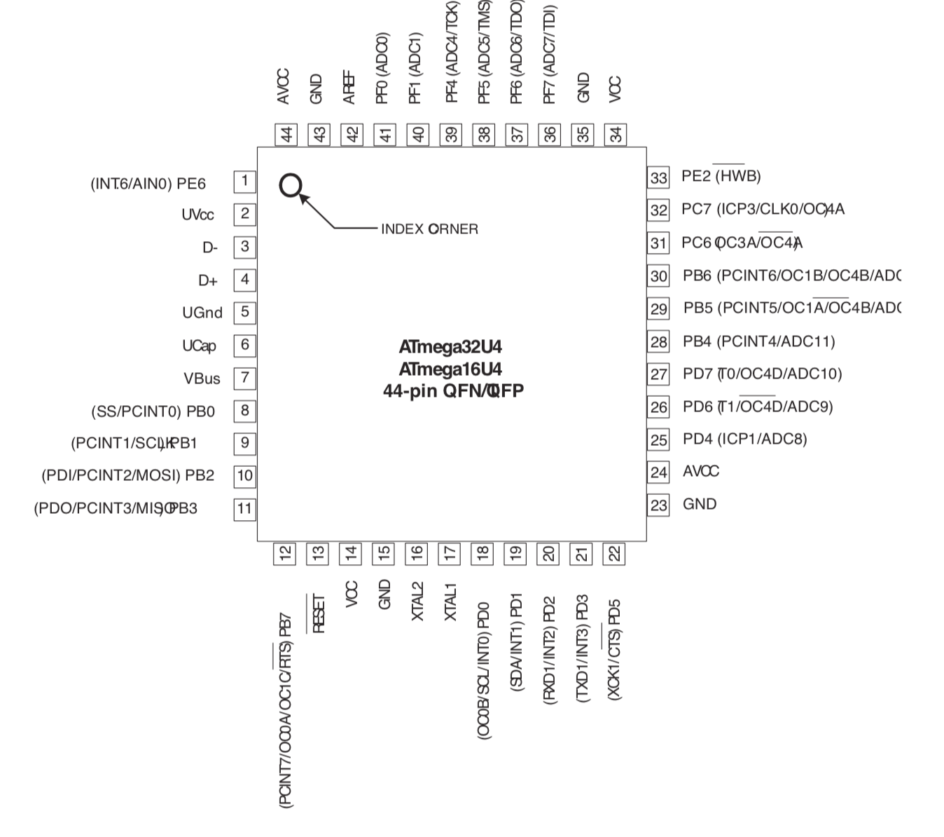
With this in mind, if I want to minimize the length of the D+/D- paths, and considering that the MCU will stay behind the space bar at the bottom of the PCB and the USB port at the top, I will have to put the D+/D- pads face up. With this orientation, this means that:
Since the MCU will be on the back of the PCB, when looking from the top, then it is possible to assign col0 to col4 to bottom right pads (which will be left as seen from the bottom), col5 to col6 to the right pads, col8 to col14 to the bottom left corner. The rows can be connected on the PFx pins on the right.
Of course this is an attempt that will serve as a guide during the PCB layout. There are great chances that I’ll have to come back to the schema to reassign columns or rows to the MCU pins as I see fit.
Here’s the schema with the rows and columns connected:
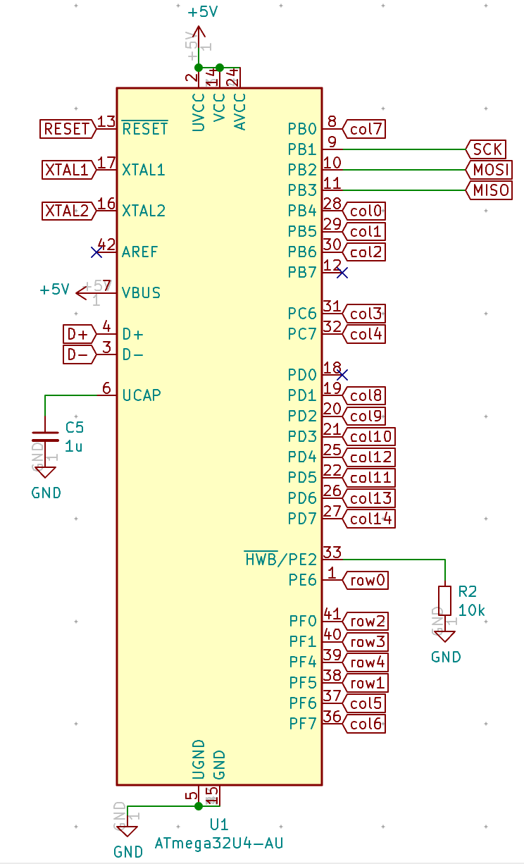
Before moving forward, I need to make sure everything is connected correctly. Kicad contains a tool called the Electrical Rules Checker that can help debug the schema connectivity. It is available in the Inspect menu.
The ERC shouldn’t display any error except a few about missing power. The ERC is complaining that our power nets (+5V, Vcc and GND) are not connected to real power sources. In fact all come out of the USB connector, but Kicad doesn’t know that this connector provides a source of power (or ground).
Hopefully there’s a way in Kicad to artificially tell those symbols are connected to a real power source. Those sources need to be connected to the special PWR_FLAG power symbol. Press the q shortcut to place a power symbol, and search for PWR_FLAG:
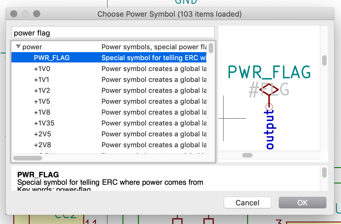
Place it on a wire connecting to GND, then place another one for Vcc and +5V:
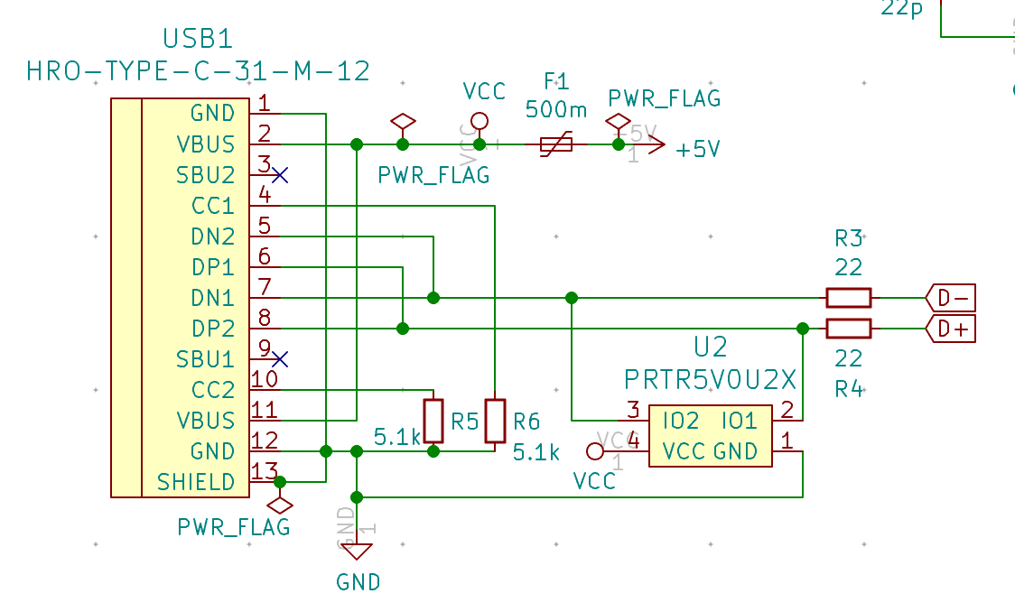
With those PWR_FLAG symbols in place, the ERC doesn’t report any errors anymore. I’m relatively confident the schema is right, but I suggest, if you also design a keyboard to double-check (and even triple-check) or ask someone in the community to check it for you (you wouldn’t want to receive a PCB that has a design flaw and that doesn’t work.)
Up until now I’ve only talked about the electronic symbols. Serious things are still ahead. In this step, I’m going to assign footprints to the components of our electronic schema. A component footprint is a physical layout describing how the component will be soldered on the PCB (that’s actually a bit more than that). For instance, for a normal through-hole resistor, the footprint will have 2 holes surrounded by soldering pads spaced at a normalized distance, the same for IC or SMD components.
This project will only have SMD components (because they are much smaller). SMD components are soldered directly on the PCB. On the other hand I want to be able to solder them with my usual soldering iron and not a reflow oven or an hot-air gun. That means I have to choose SMD components that are big enough to be able to do that easily.
For passive components like resistors, capacitors, etc, there are several normalized sizes. From bigger ones like 1206, 0805, 0603, 0402, or even 0201. In fact this number represents the size of the component in inches (centi-inches even), so for instance 1206 means a length of 0.12 inch and a width of 0.6 inch (which makes them the large). It is relatively easy to hand-solder 1206 and 0805 components with a regular iron solder (I’ll explain the techniques in a subsequent post), but not so much for the smaller ones. Soldering such components requires a magnifying glass, a pair of tweezers and soldering flux at the very least.
Here’s the exact size of those different components:

For this PCB, I’m going to choose the 0805 (and not 1206 as I originally wrote) size so that it’s still easy to solder the components but allows routing traces around the MCU. Other components have different packages of different size too. For instances, diodes exists in SOD323, SOD123, MiniMelf packages etc. SOD123 packages are much easier to solder than MiniMELF packages, because MELF components are cylindrical (and they tend to roll or misalign easily).
Let’s assign footprints to the components now. Go to the Tools menu and choose Assign footprints:
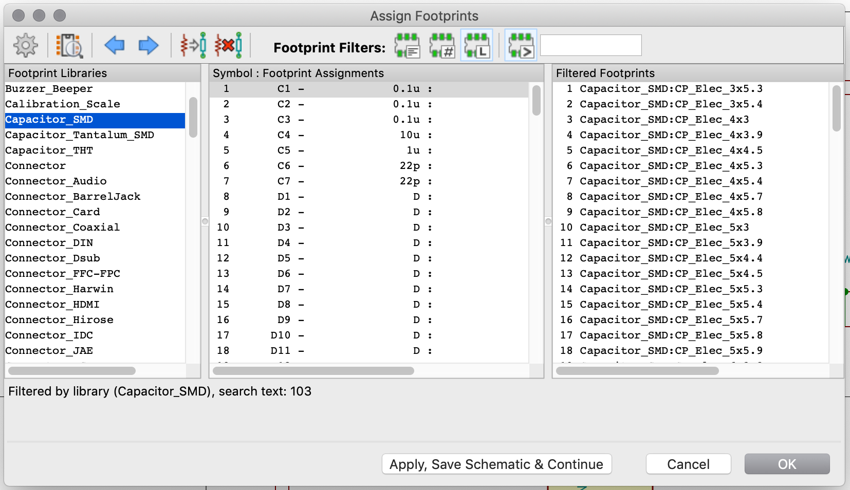
This dialog shows on the left column all the component classes, on the middle our components and on the right the individual footprints.
The task is to assign a given footprint to the references. With this, we can assign footprints in bulk, but it is also possible to assign a footprint to a given component directly from the schema by editing it (shortcut e).
As said earlier, let’s assign a 0805 footprint to our capacitors. Select all C references at once, select the Capacitor_SMD class in the left column, and select the Capacitor_SMD:C_0805_2012Metric_Pad1.15x1.40mm_HandSolder footprint. I specifically chose the HandSolder variant, because the pads are a bit larger than a regular 0805 (in fact you can almost place a 0805 component in one pad of such footprint).
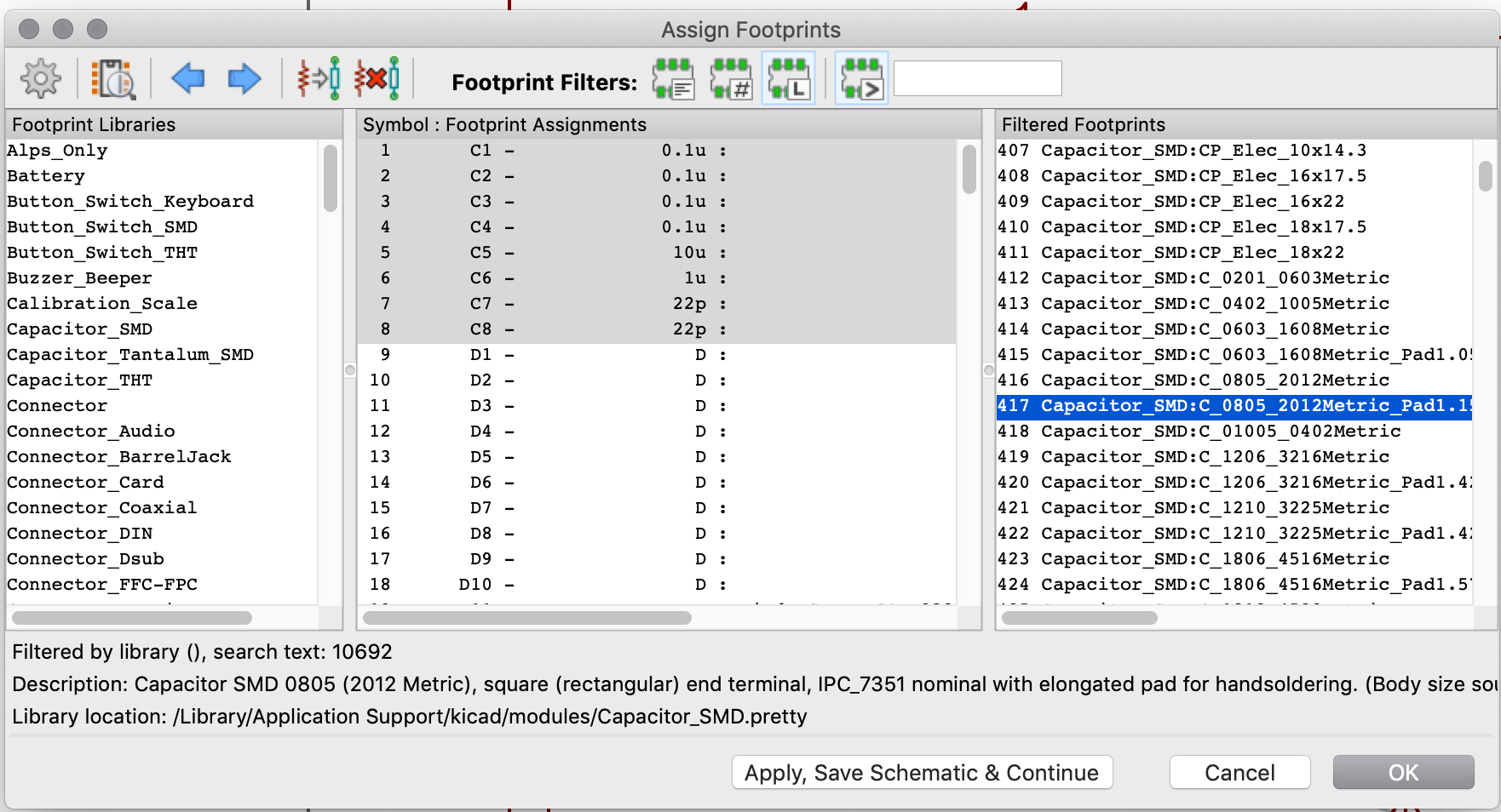
Do the same for the other components, and assign (use the search function to find the specific parts):
| Component | Footprint | Comment |
|---|---|---|
| Diodes | Diode_SMD:D_SOD-123 |
|
| 500mA Fuse | Fuse:Fuse_1206_3216Metric_Pad1.42x1.75mm_HandSolder |
|
| ISP header | random-keyboard-parts:Reset_Pretty-Mask |
|
K?? switches |
Alps_Only:ALPS-1U |
we’ll come back later to this |
| Capacitors | Capacitor_SMD:C_0805_2012Metric_Pad1.15x1.40mm_HandSolder |
|
| Resistors | Resistor_SMD:R_0805_2012Metric_Pad1.15x1.40mm_HandSolder |
|
| Atmega32U4 | Package_QFP:TQFP-44_10x10mm_P0.8mm |
it should already be assigned, but just in case |
| Reset push button | Button_Switch_SMD:SW_SPST_SKQG_WithStem |
|
| PRTR5V0U2X | random-keyboard-parts:SOT143B |
|
| USB Type-C connector | Type-C:HRO-TYPE-C-31-M-12-HandSoldering |
|
| Crystal | Crystal:Crystal_SMD_3225-4Pin_3.2x2.5mm_HandSoldering |
As an astute reader you might have noticed that I assigned 1U variants to all our switches, but that the library contained all the standard key sizes. Ai03 library contains footprints for the exact size of the various keys available on a keyboard which greatly simplifies laying out the switch footprints on the PCB. For the MX variants, larger keys also contains the PCB holes for the stabilizers. Because the references I attributed to the switches don’t tell which key it is, it’s relatively hard to assign the correct key size footprint directly from the Assign footprints dialog box. Instead I’m going to edit the handful keys larger than 1U directly from the schema, by pressing e on the switch symbol and assigning the following footprints:
| Key | Footprint |
|---|---|
| TAB | Alps_Only:ALPS-1.5U |
| CapsLock | Alps_Only:ALPS-1.75U |
| LShift | Alps_Only:ALPS-2.25U |
| LCtrl | Alps_Only:ALPS-1.5U |
| LAlt | Alps_Only:ALPS-1.25U |
| LCommand | Alps_Only:ALPS-1.5U |
| Space | Alps_Only:ALPS-6.5U |
| RAlt | Alps_Only:ALPS-1.25U |
| RShift | Alps_Only:ALPS-1.75U |
| Enter | Alps_Only:ALPS-2.25U |
| Backspace | Alps_Only:ALPS-2U |
| \| | Alps_Only:ALPS-1.5U |
To double-check, reopen the Assign footprints dialog box and make sure everything has a footprint.
The schema is now ready to be laid out on the PCB. The rest of the work will happen in the PCB layout program that is called pcbnew in Kicad. You can start it from the schema editor by clicking on the PCB icon in the toolbar.
This will open the PCB editor with a blank view and grid. Do what ai03 suggests in his guide to setup the user grids: create a user grid settings with X: 0.79375 mm and Y: 0.79375 mm (make sure to be in mm, refer to ai03’s guide for the complete instructions):
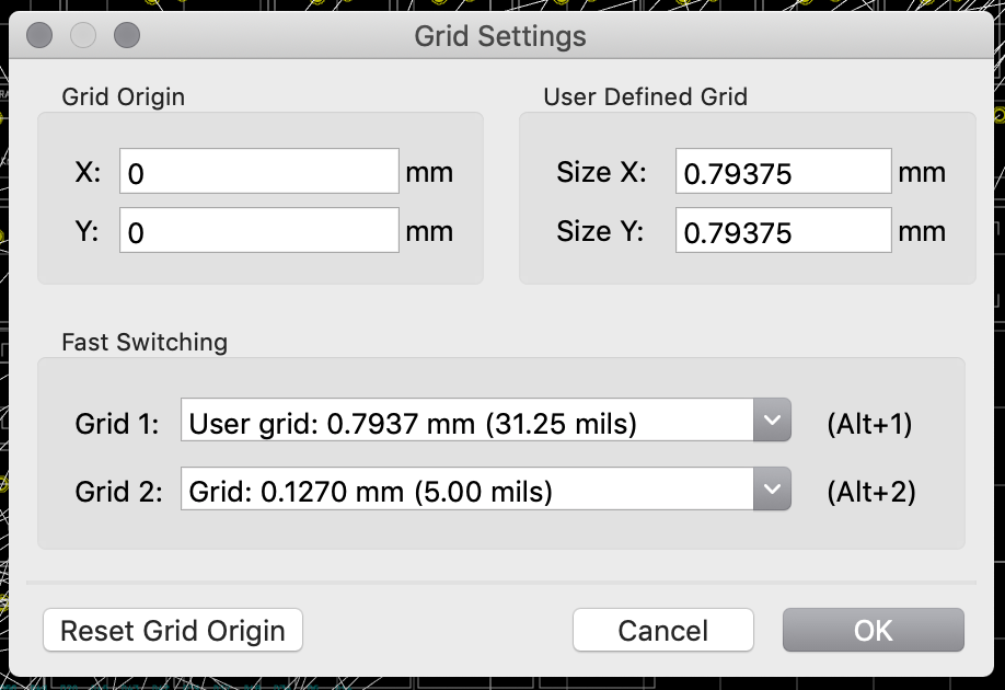
Copper tracks have resistance. This means that a track has a voltage drop, power dissipation, and a temperature rise when current flows through it. The resistance is a function of the track length, width, thickness and of course resistivity of its material.
For signal tracks (like the matrix), there’s very few current involved, we can keep the Kicad default (0.25 mm or a bit less than 10 mils). The usual advice is to make the tracks as large as the design allows. A keyboard by definition has a large PCB. Since there’s no led nor any features other than the switches and the electronic components, this PCB will be reasonably empty. It’s a good news: we can make the power tracks as large as we need. By power tracks I mean in fact the +5V, VCC but also GND. In fact, GND is as important as the other power signals because it will carry all the return currents from the ICs, and thus is subject to as much current as the other power nets.
So power tracks are required to be larger, but what size do we have to use? Ai03 in his guide suggests 15 mils. This sounds right, but in fact there is a way to compute the exact track width. Unfortunately determining trace width is a complex science. The IPC has published a (paying) standard, IPC-2152. IPC-2152 publishes an abacus that allows to find the trace width based on projected current, copper thickness and temperature rise. Hopefully we can also use one of the numerous PCB trace width calculator.
Copper thickness on PCB is measured in oz/ft2 (looks like the metric system lost again). The default is usually 1 oz/ft2. If we have 500mA, default 1oz/ft2, and a maximum temperature rise of 5ºC (we don’t want the temperature to increase too much), the calculator returns 7.1 mils in open air, or 18 mils for inner layer trace. The IPC-2152 standards does it’s calculation with tracks spaced by 1 inch. This isn’t really practical for a real life PCB, so we might just want to aim for a smaller temperature rise (two parallel tracks at 500mA will increase temperature more than only one) to 2ºC (another solution could be to increase the projected current as if we had more current in one track simulating two close tracks). The result is a trace width of 12 mils.
Of course nothing is perfect, and the copper traces might contain debris or be etched. Any of those modifications will increase the trace resistance, and thus the temperature rise. Because this keyboard will be in a closed unventilated case, we need to limit the temperature rise as much as we can afford (remember that the MCU will also produce heat). Because of that, I’m going to add a safe margin and use 15 mils (as ai03 suggested) for the power traces.
Doing the same reasoning in reverse we could also reduce the size of the signal traces. Most manufacturer nowadays can do 5 mils (0.127 mm) traces. We have plenty of space on this keyboard PCB, and it costs the exact same thing if we do 5 mils traces or 10 mils traces, so let’s keep the default 10 mils.
Kicad has a feature that allows you to declare trace width based on the net they’re built for (ie connections between components). This allows to automatically adapt the trace width depending on if the route is for power or signal. This can be done in the File → Board Setup dialog box, section Design Rules → Net classes.
Click on the + sign to add a class called Power, and adjust trace width to 15 mils (you have to be in inches mode to do that). Then in the bottom part of the dialog box, assign this power class to the VCC, +5V and GND nets:
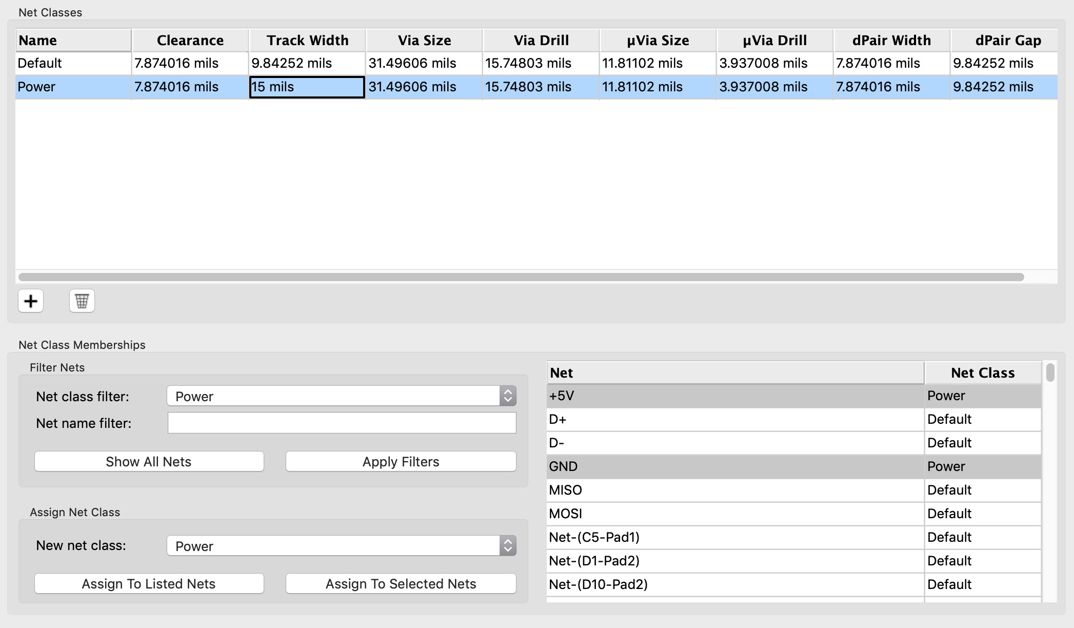
Finally, let’s import the components to the PCB by going to Tools → Update PCB from schematics…. This gives this pile of components:
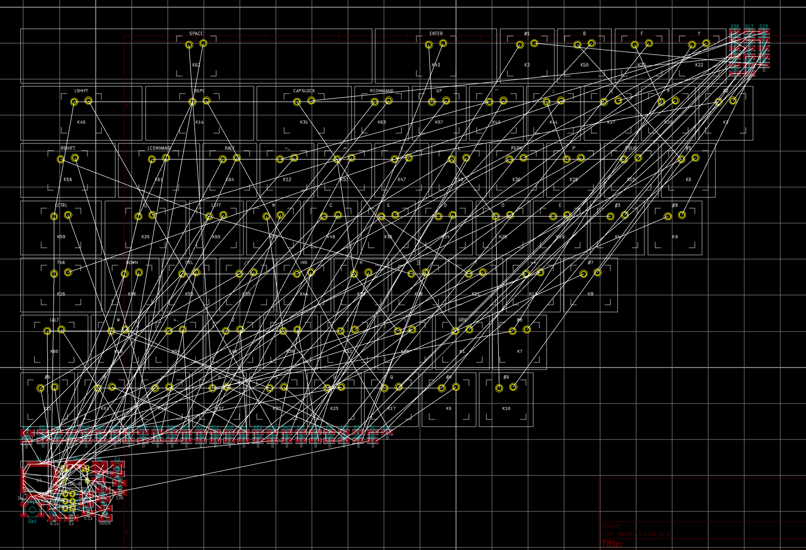
You might notice all the components have been packed together (all the keys, all the diodes, etc). If you zoom in on the components, you’ll notice that their pads are all drawn in red. This means those components are laid on the top of the PCB. This is the perfect time to talk about PCB layers.
A PCB is a dielectric board usually made from FR4 fiberglass. Copper planes are sandwiching this board, on which the traces are drawn. There can be one layer, 2 layers (one at the top, one at the bottom), 4 layers (2 on top separated by a dielectric substrate, and 2 at the bottom), 6 layers, etc. Each couple of layers increases the manufacturing price. For this keyboard, a 2 layers PCB will be enough.
Kicad defaults to two layers boards (you can add more if needed), one on top (the red one) and one on the bottom (the green one), they are respectively named: F.Cu (Front copper), and B.Cu (back copper). But Kicad also defines other layers:
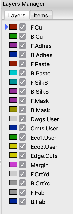
Here is a table summarizing their usages:
| Layer name | Type | Usage |
|---|---|---|
| Cu | Technical pair | Copper layer for traces |
| Adhes | Technical pair | application of adhesive to stick SMD components to the board prior to soldering |
| Paste | Technical pair | mask to place solder paste for reflow soldering |
| SilkS | Technical pair | where the components are drawn |
| Mask | Technical pair | defines the areas free of soldermask like component pads |
| CrtYd | Technical pair | show how much space a component physically takes |
| Fab | Technical pair | documentation for manufacturing |
| Fab | Technical pair | documentation for manufacturing |
| Edge.cuts | Independent | the board shape |
| Margin | Independent | to define a safe margin for edge cuts |
| Dwgs | Optional | can be used for instructions, drawings. Some footprints use them |
| Cmts | Optional | can be used for instructions, drawings. Some footprints use them |
| ECO1/2 | Optional | user specific, never used in footprints |
Since this PCB will have two layers, it would be possible to evenly spread the components on both layers. Since there are much more room on the back (all the switches take space on the top), it’s preferable to put all the SMD components on the back (bottom layer). Also, putting all the components on the same layer would reduce the manufacturing costs if I wanted to order soldering. Note that this will also reduce the number of vias (a via is a hole in the PCB that connects electrically two layers).
First let’s move all SMD component footprints to the B.Cu layer. To do that drag select the components and press the f shortcut (to flip them to the other face). If they get placed on the way or far away, press m to move them closer.
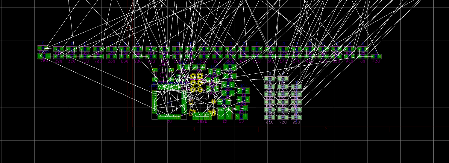
The most difficult task in designing a PCB is routing the copper traces between components. Those traces should be carefully designed to prevent EMI (I’ll talk about that in a subsequent post), not cross layers too many times etc. Routing is an iterative process that is very time consuming, and can be considered as an art (at which I’m a newbie, you’ll see that soon). But before we can start routing the PCB, we need to place the components. Laying out the component is more than half of the routing work. Components badly placed can make routing hard or impossible.
Some components can’t be placed anywhere, think for instance of the switches that need to be placed where the keys will be. Same for the USB-C connector. Then other components might have constraints that also mandate where they are, for instance the decoupling capacitors that need to be close to the MCU to be effective.
I’m going to start with the key switches because that’s them that will define the size and aspect of the PCB. Let’s switch to the User Grid 0.7937 mm which has been designed to place switches. This grid is 1/24th of a key. The task is to move every switch footprint in the order of the layout of the final keyboard, starting with the GRV key. With this User Grid in place, the switches will snap together perfectly. It is also possible to use the arrow keys to move the components in place.
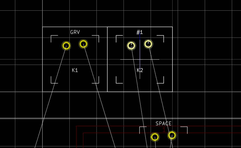
Keep going until all the keys form the layout. Note that the key name (which we put in the component value earlier) appears on the footprint. This simplifies the placement of the switches.
If you struggle to find a key, you can use the Find functionality (Ctrl-F) and enter the key reference. Even better use the t shortcut to activate the Get & Move Footprint feature, enter the reference, then move it to the right place.
Here again it is easy since we’re laying out the keys in order of increasing K? reference (from K1 to K67). Make sure all switches outer white bounds are aligned when placing a new key next to an already placed one. Their borders should only form one thin white line. It might be easier to hide the rats-nest while placing the switches (there’s a button in the left vertical toolbar to do that).
In no time you’ll get the whole matrix properly aligned:
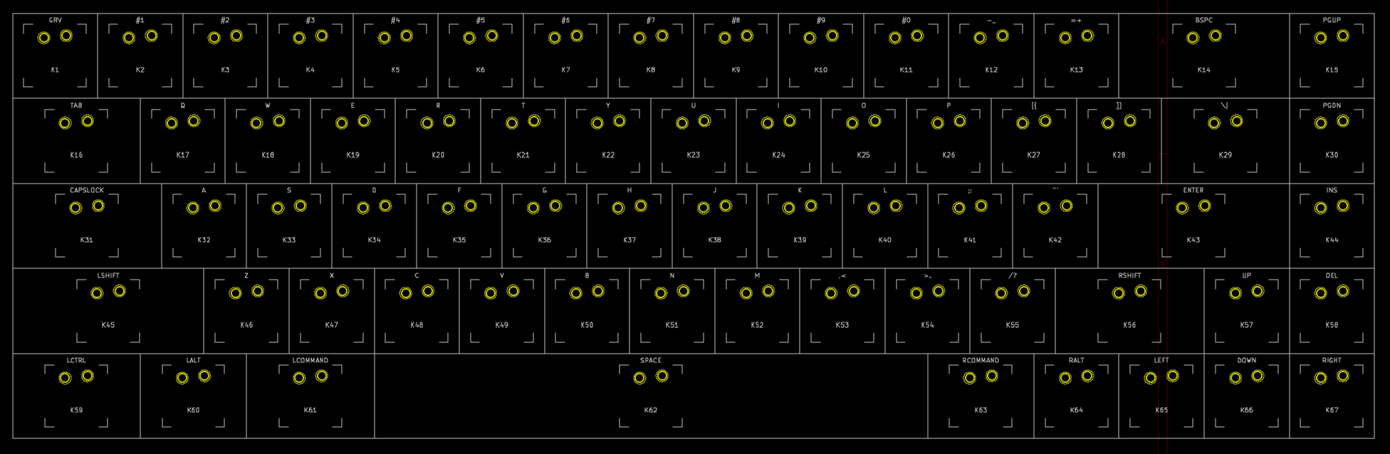
In the process of aligning the keys, I noticed that I misattributed the footprints of two keys. To correct such mistake, you need to go back to the schema, change the footprints to the correct ones (by editing the components). Next go back to the PCB editor and click on the Tools → Update PCB from schematics…. In this dialog box, make sure to select the Update footprints and the Reassociate footprints by reference method. The misattributed footprints should be corrected automatically.
The next step is also quite tedious. It consists of moving all the diodes to their parent switch positions (by using the t shortcut). Still with the switch User Grid, start with D1, move it to the K1 position, rotate it as you see fit with the r shortcut. Do the same for D2 and so on:
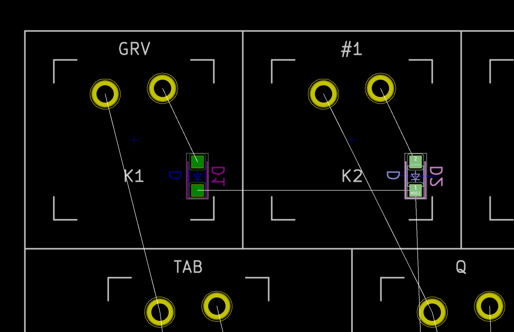
It’s best to do this part with the rats-nest visible. The rats-nest is the forest of white lines that connect all pads part of the same net. It’s a visual help used during trace routing. In the diode layout phase it also helps visualize rows and columns. For instance in the picture above, D1 pad 1 and D2 pad 2 are connected to form a row.
Once done, the result looks like that (the entropy has greatly declined !):
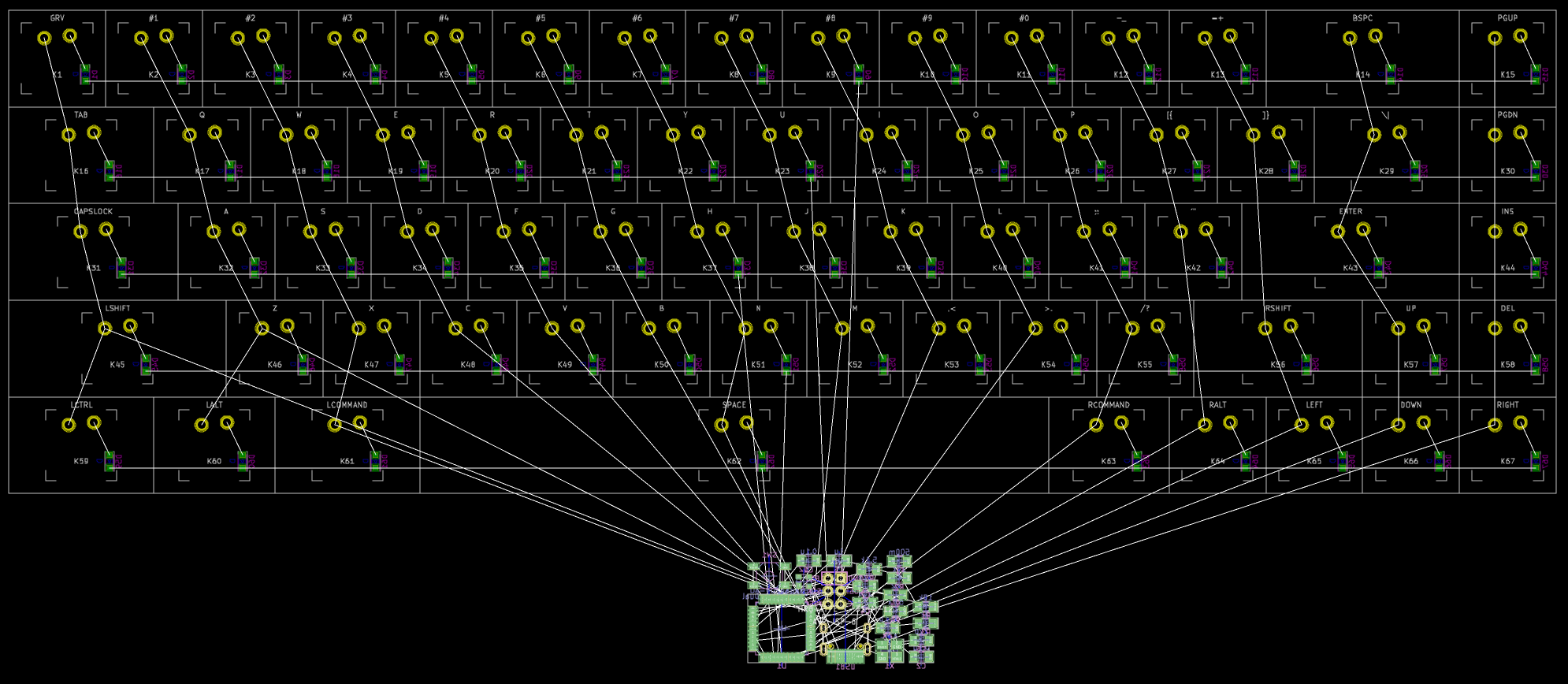
The next components to lay out is the USB Type-C connector and its associated components (like the fuse, the ESD protection IC, etc).
There are different schools regarding where to place the USB connector. I find centered connector to be more appealing visually. Still with the switch User Grid settings, move the connector to the center top of the board (which happen to be between the 7 and 8 key):
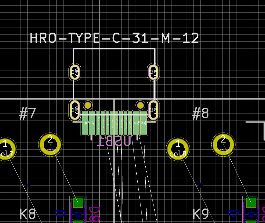
Since the footprints hotpoint is exactly at the center, and thanks to the switch User Grid Settings, it is easy to perfectly snap in the connector between two keys.
Next, we’ll move the components that needs to be close to the USB connector there. It means both 5.1k resistors, the PTC fuse and the ESD protection device. Notice how I carefully placed those to minimize the number of nets crossing:
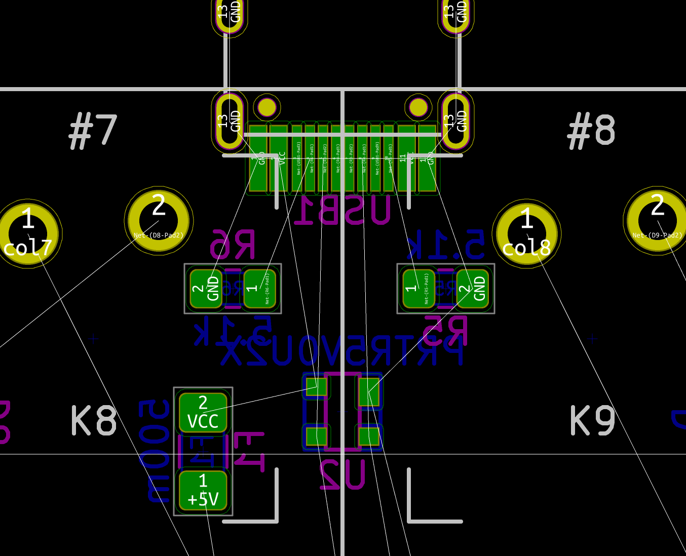
Now, I need to take care of the MCU and the components that are connected to it. The MCU is quite large, but hopefully there is enough room between the space key switch and the other switches. Ideally we have to route the D+/D- differential pair with the shortest path possible (to control the USB data-lines impedance). The crystal also needs some room. It looks like the best way is to orient the MCU with the D+/D- pins face up and the crystal to it’s right. Of course, things will probably change when I’ll start routing:
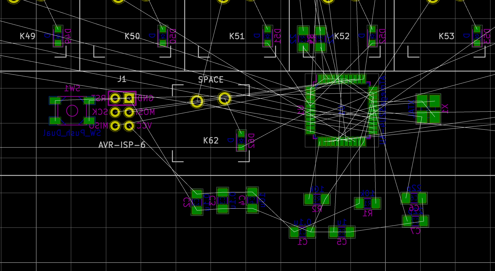
Around the MCU, there are so many nets that it might be hard to see what’s connected to what. At any time it is possible to highlight a net by using the Highlight net function (shortcut \`). For instance to better see the nets around the crystal:
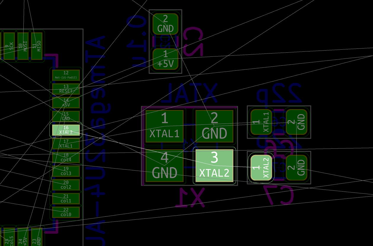
The crystal needs to be connected to the two 22pF capacitors and the two XTAL1 and XTAL2 pads on the MCU. The following arrangement allows to take advantage of the free space around the MCU while minimizing the number of crossing nets and leaving room for routing the matrix around:
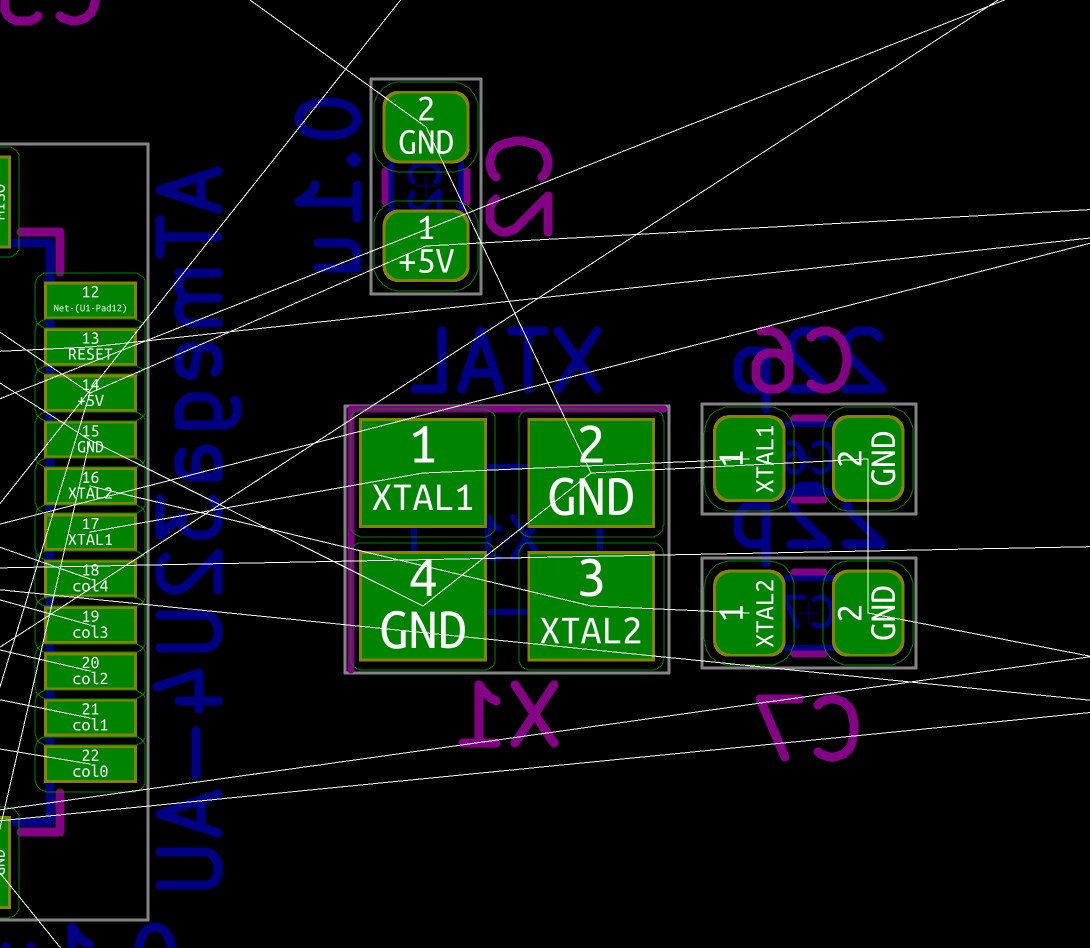
The D+/D- differential pair (the USB data lines) requires two 22 ohms resistors to make sure the USB bus is terminated with the correct impedance. Those have to be placed as close as possible to the MCU. We can orient them in the direction of the USB-C connector:
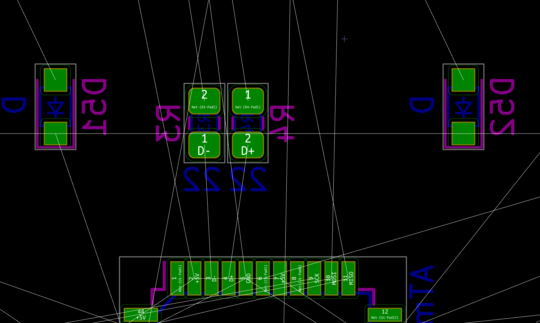
The next step is to add a decoupling capacitor for each VCC pad of the MCU. We’ll keep the 10uF capacitor close to UVCC and VBUS as I explained in the first part. The rest of the 0.1uF capacitors will be moved close to the other VCC pins. The idea again is to minimize the number of nets crossing while still leaving room for routing traces. We also do the same for the RESET pull-up resistor, the UCAP capacitor and the HWB resistor, and finally the reset push button:
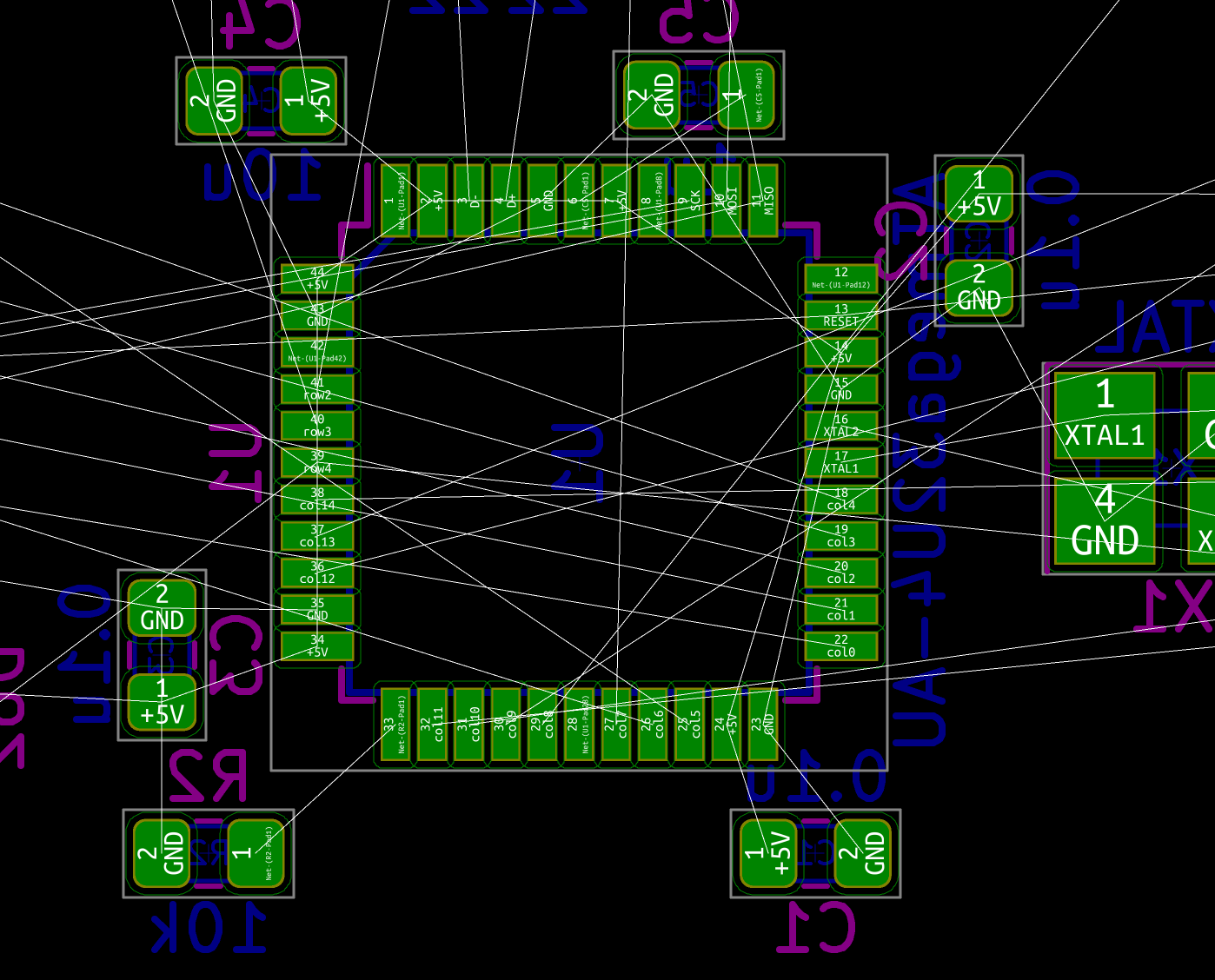
As said earlier, this is a tentative layout. When I’ll start the routing, there are very good chances that I’ll have to move things a little. Note also that I haven’t placed the ISP header. I’ll do that during routing, because the matrix might not be hooked exactly like we did above in the end, and I might reuse the MISO, MOSI or SCK pins for the matrix.
The board now looks like this:
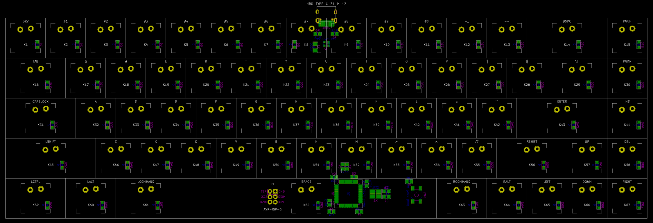
Notice that all components are now placed inside the switch footprints, thanks to the SMD components small size.
Now that everything is approximately at the right place, we can design the PCB border. In order to do that, I’m going to draw the contour while being in the Edge.Cuts layer. This will let the manufacturer know where the board should be cut. This can be used to give specific forms to the PCB. In this case, I’m going to draw the border exactly on the key bounding boxes, including the USB connector. The HRO-TYPE-C-31-M-12 connector has four through-hole pins that needs to be soldered which means the PCB must extend under those (this will help secure the connector and prevent it to become lose while connecting/disconnecting cables frequently).
Let’s start at the top-right corner (any corner will work though), select the Edge.Cuts layer and the Arc tool. Switch to the switch User Grid settings if you’re not in it and click in the middle of the top right corner:
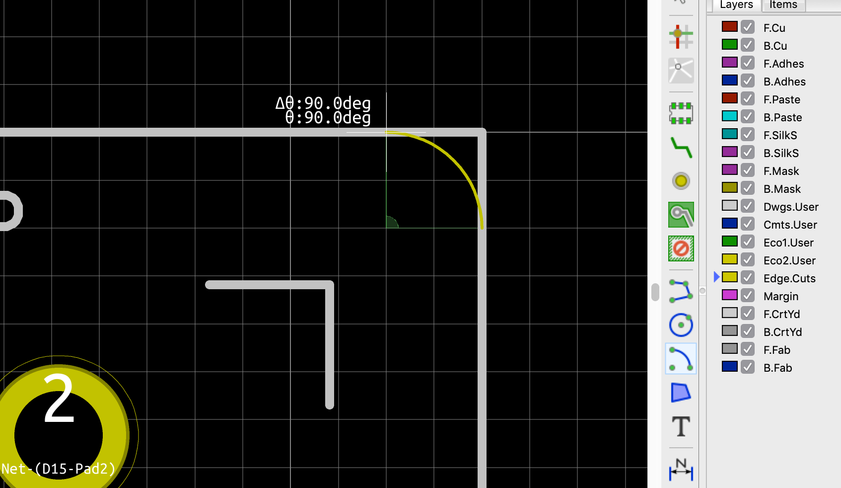
Select the arc that just has been drawn and Copy it (Ctrl-C) by clicking on its control points. Then paste the copy (Ctrl-V) and move it to the bottom-right corner (or any other corner). Rotate it by pressing r until it has the correct orientation and place it in the corner:
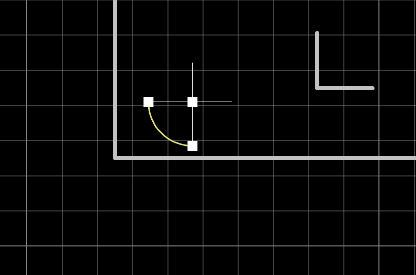
Repeat for the two remaining corners. Before adding the edge lines, I believe it’s easier to prepare the USB connector. Draw an Arc on the left part of the connector and continue it with a line:
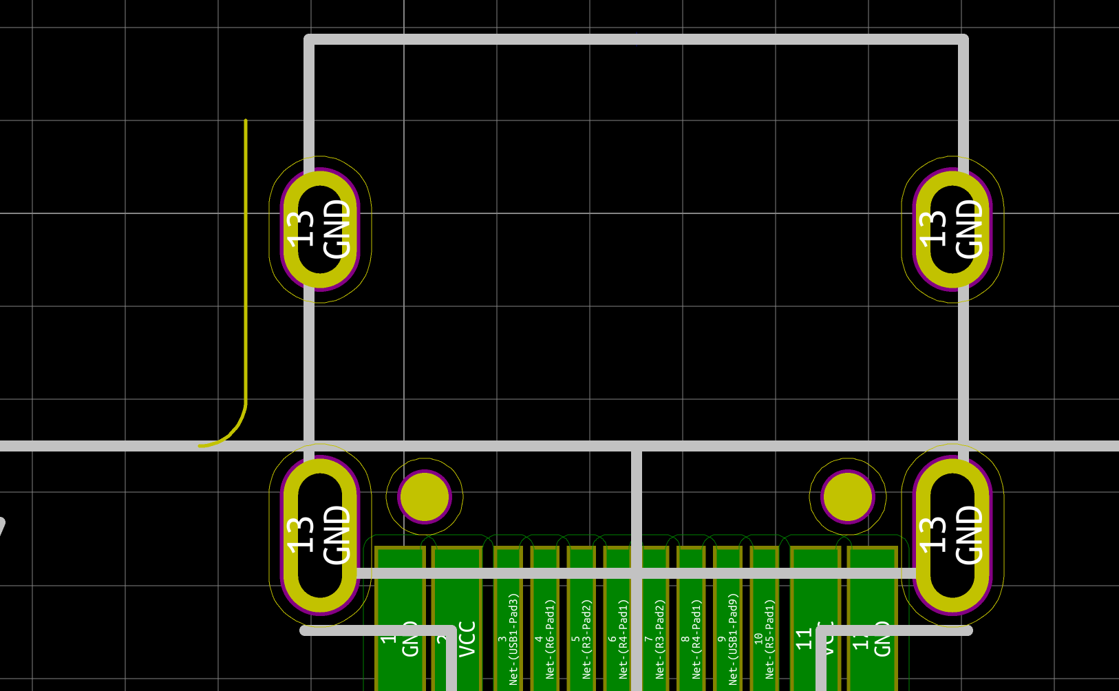
Then the draw the horizontal and right vertical edge:

And finally copy the left arc (make sure to click the the bottom left control point):
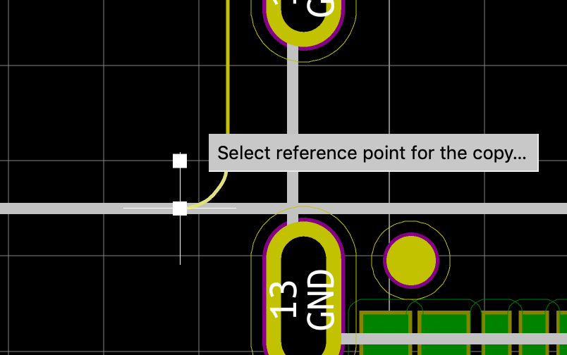
Next, move the arc to the right part of the usb and rotate it (r):
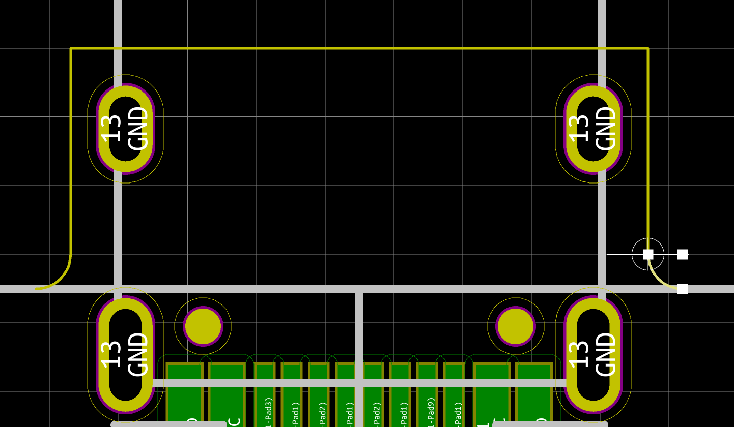
Then finish the border by drawing Lines connecting all the rounded corners:
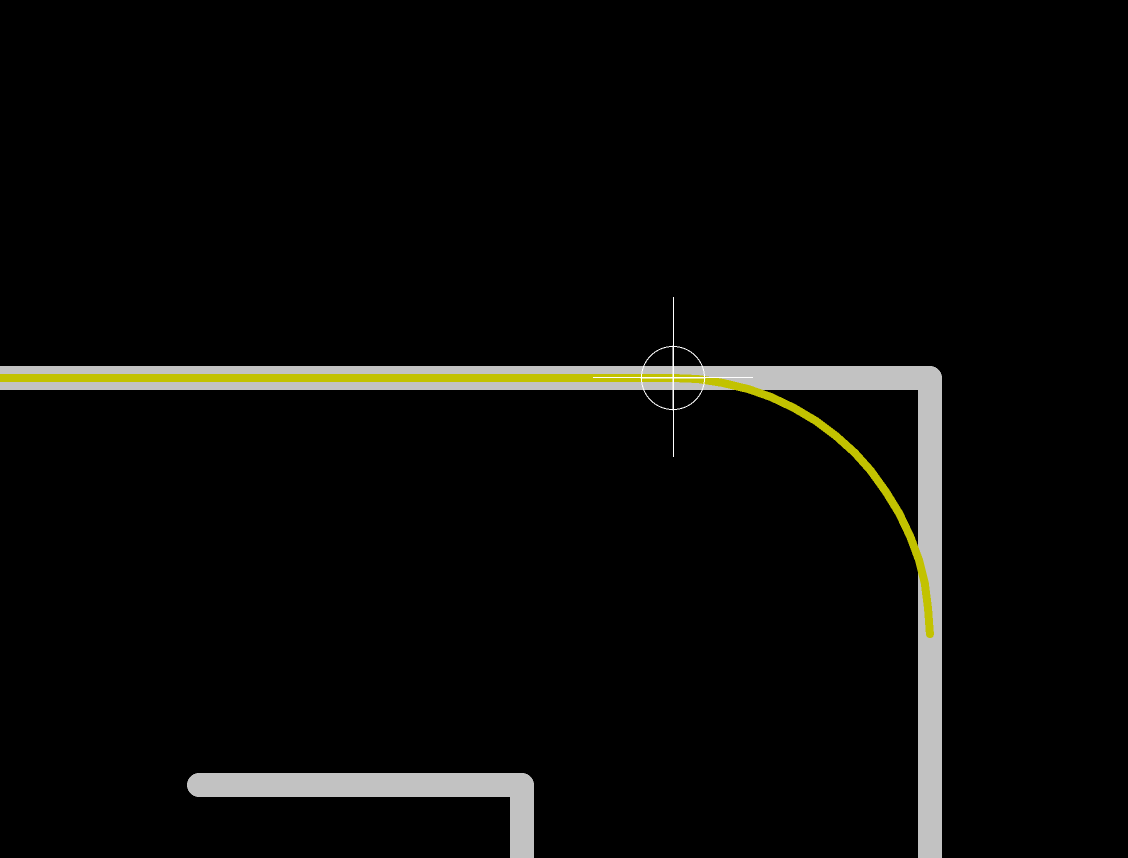
Now, inspect visually the edge cuts to make sure everything is aligned and connected. To have a better view, I recommend to hide the Dwgs.User layer (where the switches bounding boxes are drawn). I also ran the Design Rule Checker (from the Tools menu) to spot any edge cut errors:
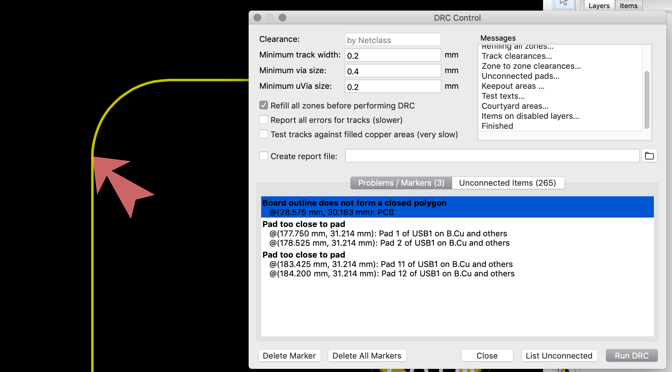
In this case the line was extending into the arc too much (by one grid step). It was easy to fix but couldn’t be found except with the DRC.
If you followed the design so far, you should have the following PCB:
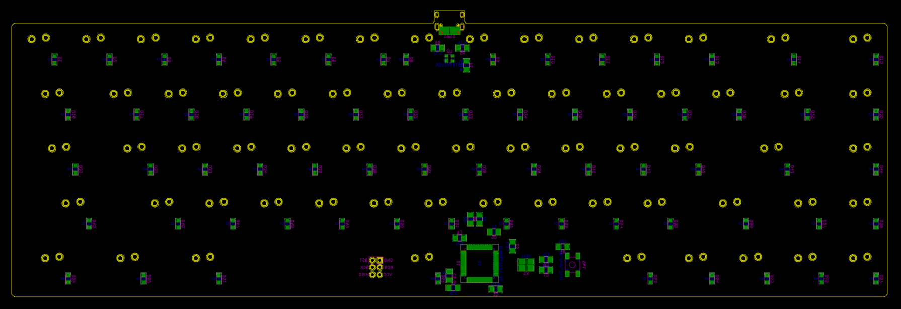
There’s a feature in the Kicad PCB editor to see the PCB in 3D. I don’t have the tracks laid out yet, but all the components have been placed so there’s something to see. Activate View → 3D Viewer to see the board top. You can rotate the board (not the best virtual ball I’ve ever used) with the mouse and see the bottom face (which contains our components). You’ll soon discover that there’s no 3D model for the USB Type-C connector. Hopefully it’s easy to add it. First edit the USB Type-C connector, then click on the Footprint Properties icon and finally click on the 3D Settings tab:
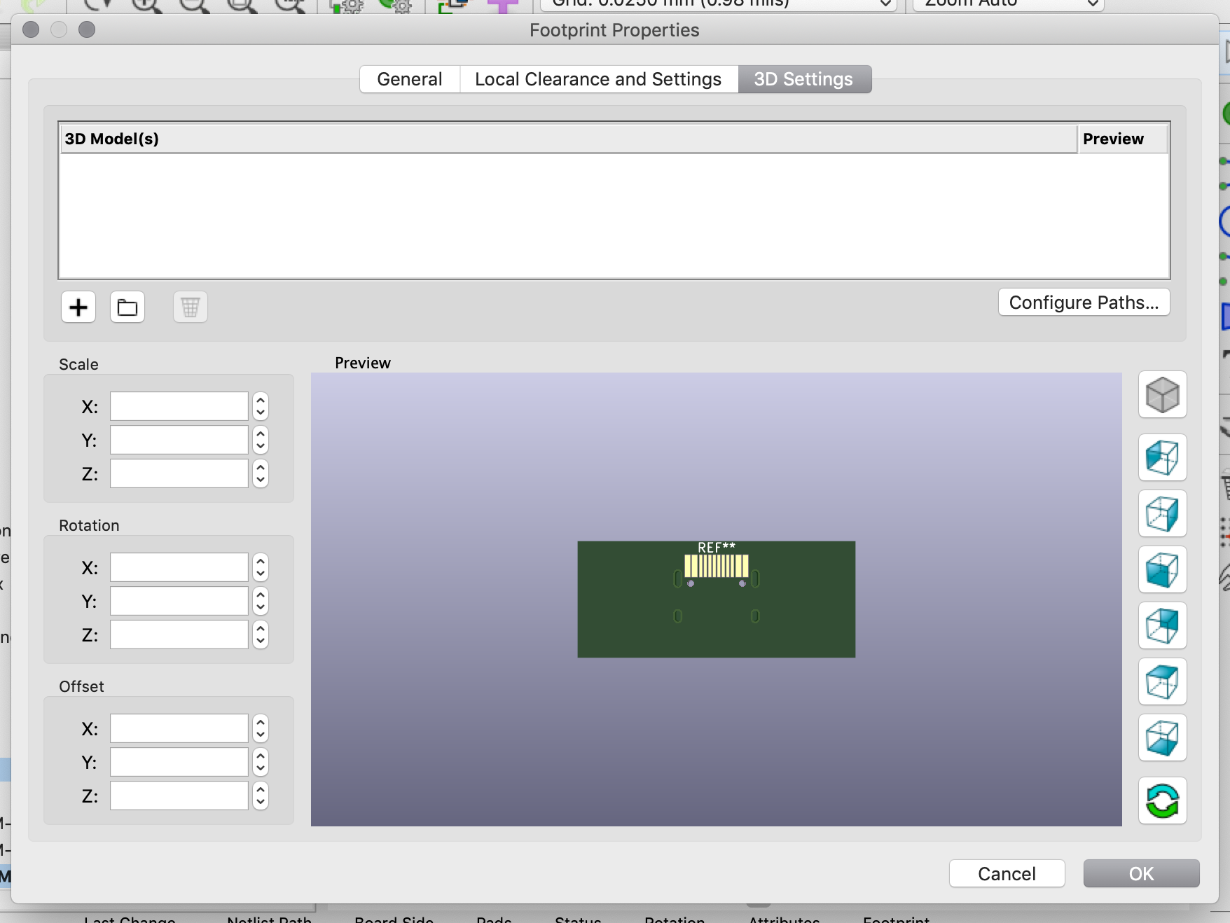
Kicad doesn’t know where to load the USB Type-C connector 3D model, click on the folder icon to add it and chose the Type-C.pretty/HRO TYPE-C-31-M-12.step file:
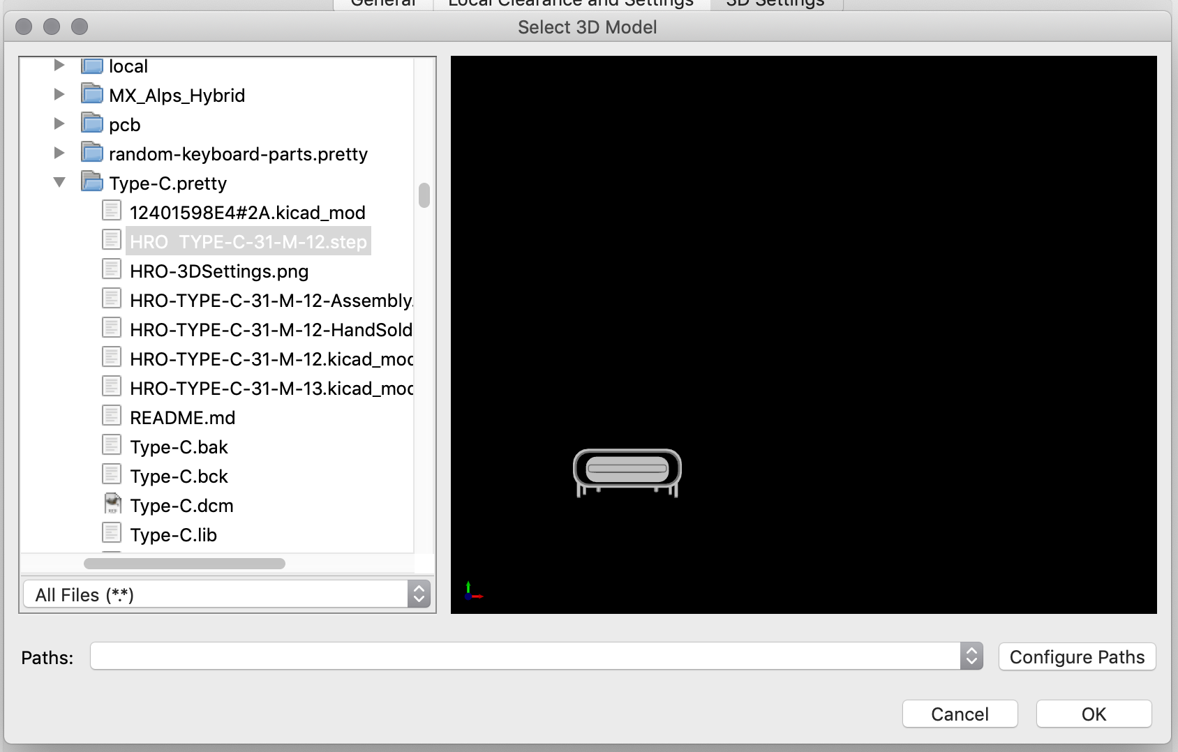
This loads the 3D model but in a completely off orientation:
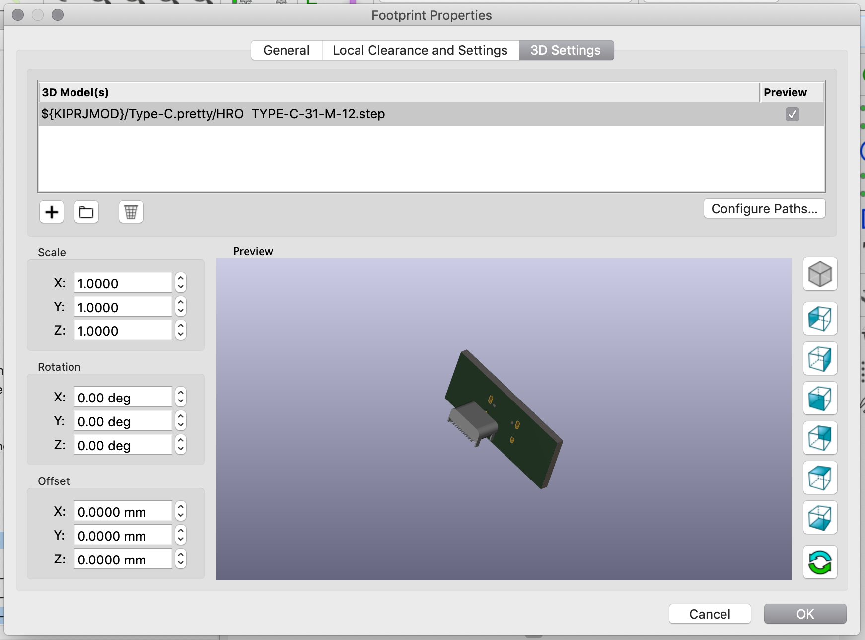
Apply the following transformation so that the connector has the correct orientation:
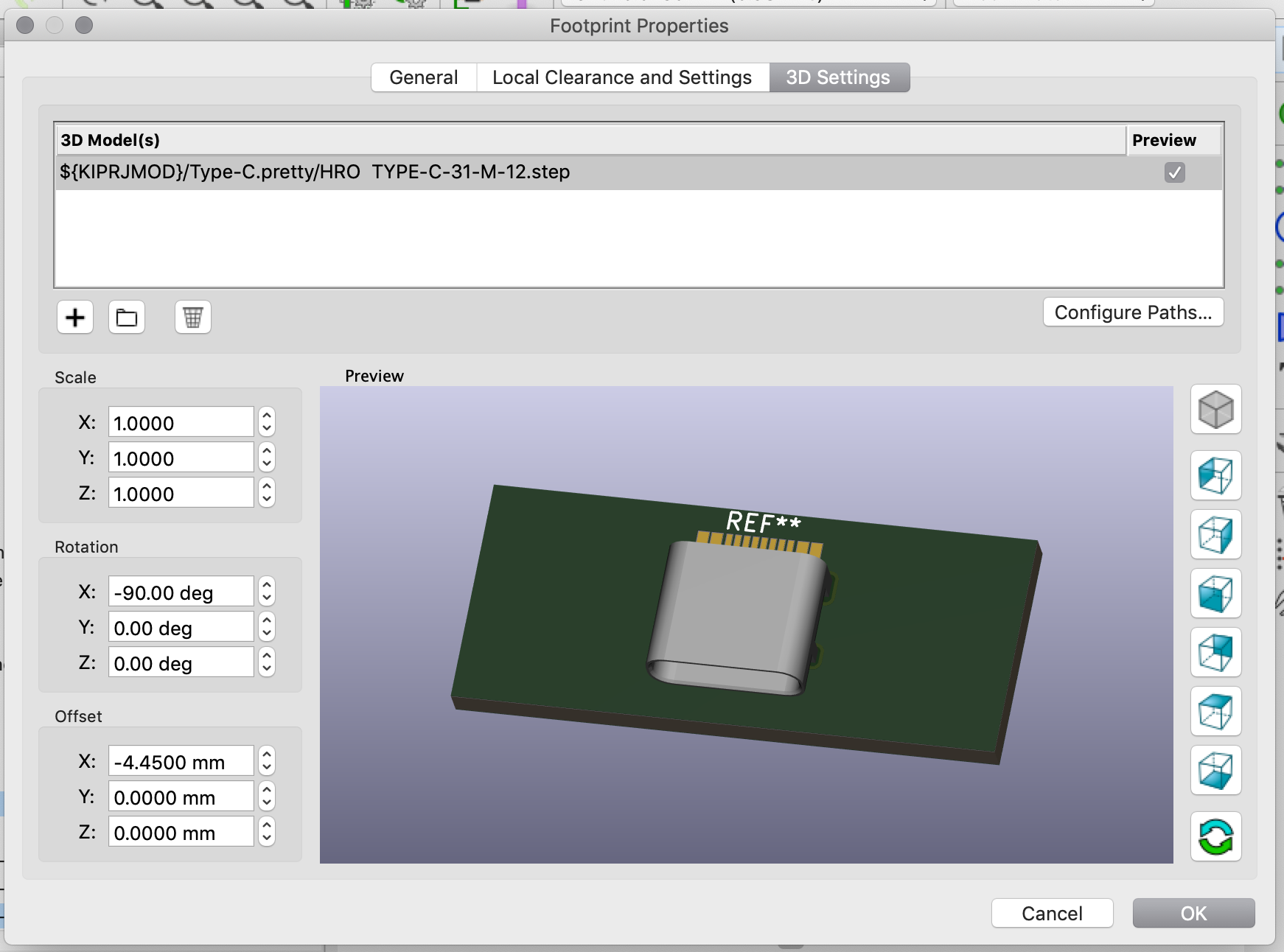
Save the footprint, and finally the board can be rendered with all the components:
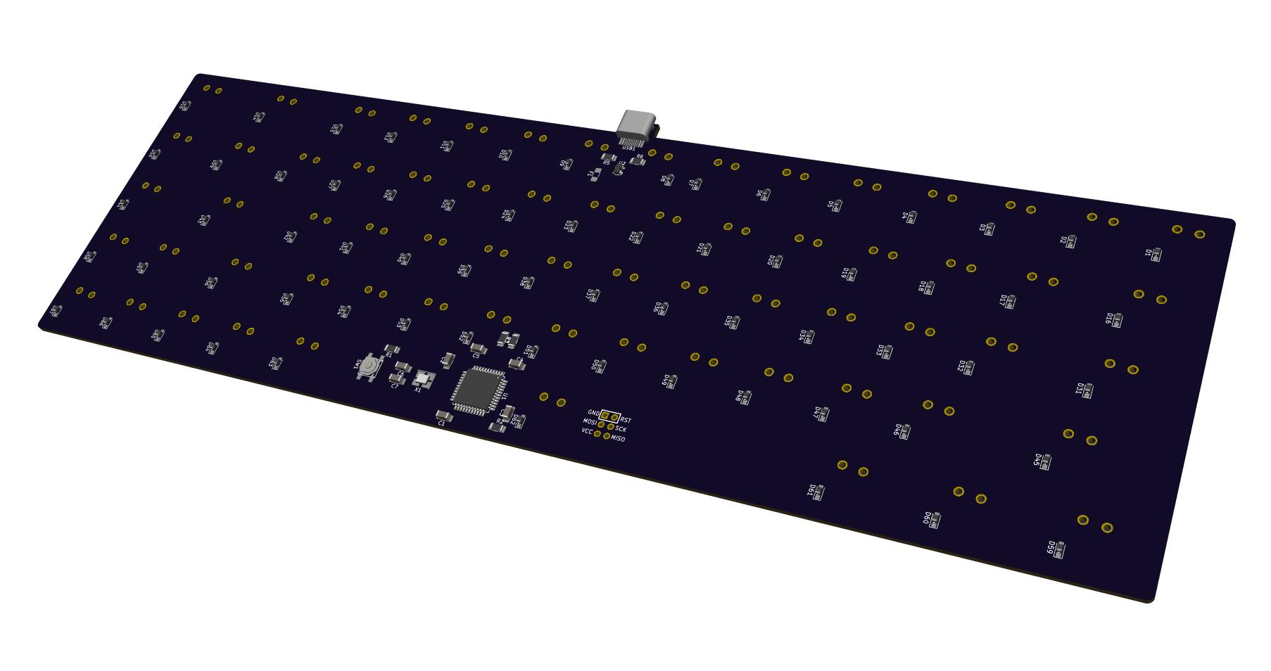
That’s all for today. We’re still far from having a working PCB, and in the next episode I’ll cover:
Thanks for following!
Want to read the next part? Then click here for the Designing a Keyboard part 3
This collection now contains the following articles:
I’ve been in the keyboard community for more than two years now and my keyboard collection is starting to fill up my shelves. It’s only recently that, as an engineer, I started to think about how keyboards were really working.
Some times ago, I got my hands on a 90s mint-condition Apple Extended Keyboard, some AEK keycaps and Alps SKCM switches. The idea I had, was to wait for a Group Buy to happen for an Alps based keyboard (like the ADK64) and then build a new keyboard with parts coming from old keyboards.
Alas, I missed all the nice Alps GB (ie the Lunar). Still I wanted to build a modern keyboard with those parts. One of the reasons is that I worked with such mechanical keyboards back in the 90s and I remember that their tactile feeling was among the best I’ve experienced.
So, an idea started to grow in my mind. What if I designed my own Alps based keyboard ? This way, I would be able to have the layout I want, instead of being forced in a 60% layout I’m not really fond of.
This series of articles will tell this adventure. My aim is to allow anyone to also start designing their own keyboards, piece by piece, but also understand how everything works.
At the time of writing, I have validated the PCB rev0, almost finished designing the case and plate, but the keyboard itself is yet not finished.
In this episode, we’ll focus on beginning the electronic schema (outside the matrix). The very next episode will focus on the matrix, assigning footprints, etc. Then we’ll have at least one episode on the PCB design.
So I said earlier that I got some Salmon and Orange Alps SKCM switches that were desoldered from an existing 90s AEK. The Salmon switches are not in a very good condition (they would require cleaning at least), but the orange ones are. I also have 2 sets of AEK keys, one in Japanese and the other one in ANSI layout (qwerty US).
The aim is to build a 65% ANSI keyboard with the following layout:

I codenamed this keyboard the AEK67 because there’s 67 keys in it, but I’m looking for a better name (any help would be very much appreciated on this front). You’ll notice that this layout is the same as the Lunar one. It also has the same issues:
The original AEK keyset doesn’t have those keys. There are possibilities of using a different key, for instance a Caps Lock, but it won’t have the right profile. The Lunar GB solved this issue by casting a specific 1.75u key in this profile, unfortunately I wasn’t able to get one. Well, we’ll see when the keyboard will be finished :)
Unlike my previous experiment at building a handwired keyboard, this time the aim is to design a full-fledged keyboard, including a PCB and a real case.
Since I needed to start somewhere, and I already had some basic electronics knowledge from my engineering degree (25 year ago), I started by designing the electronic board.
I explained a bit how a keyboard works in the handwired build log, but let’s refresh our memories. A keyboard is the combination of:
The PCB is the electronic board that converts key presses in commands that the computer can understand (that’s the HID protocol for USB). The PCB contains a micro controller (the MCU for short, it contains a CPU, a bit of RAM, flash memory and many I/O ports) and an array of switches (which form the matrix).
The switches are arranged in columns and rows to mimic the physical keys layout. At a very fast pace, the MCU will scan the matrix by providing a voltage on a given column, then the next one, etc and reading the lines.
If a key is depressed, the voltage will appear on the line of the pressed key when the MCU feeds the tension on its column, because the current will flow from the activated line to the row through the switch. The MCU deducts the key that has been depressed by looking at the rows and columns it is currently applying and reading the voltage.The MCU can then send the corresponding normalized key code on the USB wires to the computer (what the computer does is another story, sorry ;-)).
But there’s a problem: if one presses more than one key at a time, it is possible for the controller to register ghost keypresses. See the following schema of a conventional 4 switches matrix:
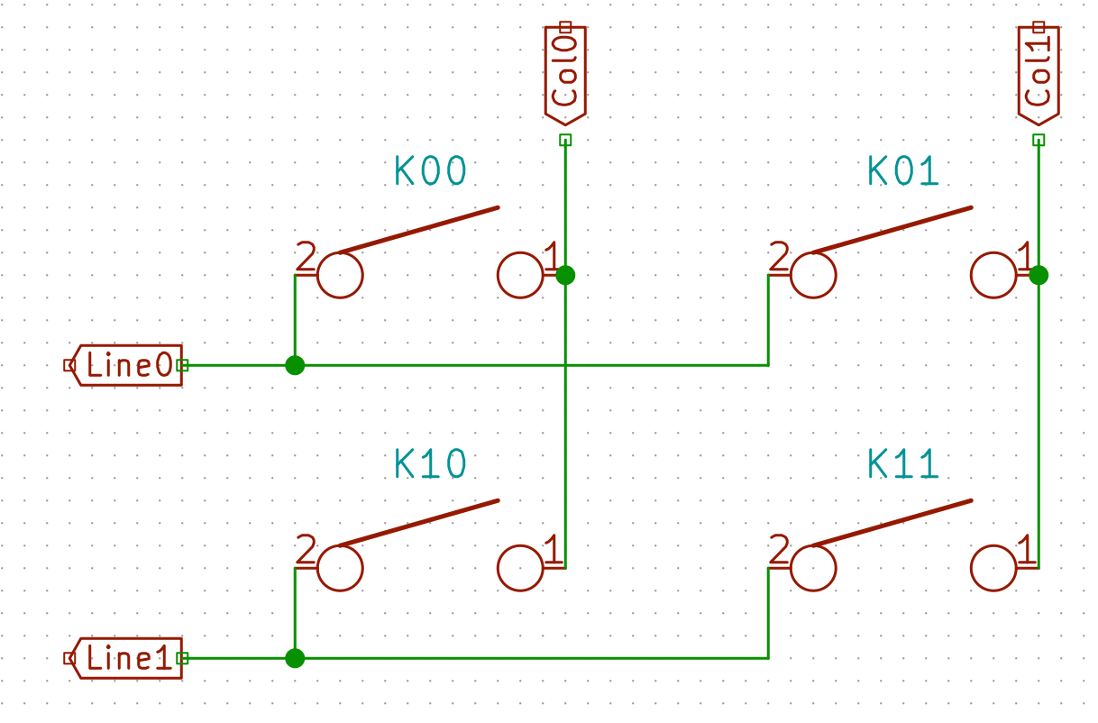
When the controller powers the Col0, and if K00, K01 and K11 are depressed simultaneously, the controller will see a tension on both Line0 and Line1, because the current will flow from Col0 to K00 pin 1, then pin 2 because the switch is closed, then to switch K01, then to switch K11, then to Line1. For the MCU it is as if all the switches have been pressed, instead of the 3 that were indeed depressed.
To prevent this we add diodes between the switch and the row it is connected to. Diodes are electronic components that prevent the current to flow in the reverse direction. The matrix becomes this:
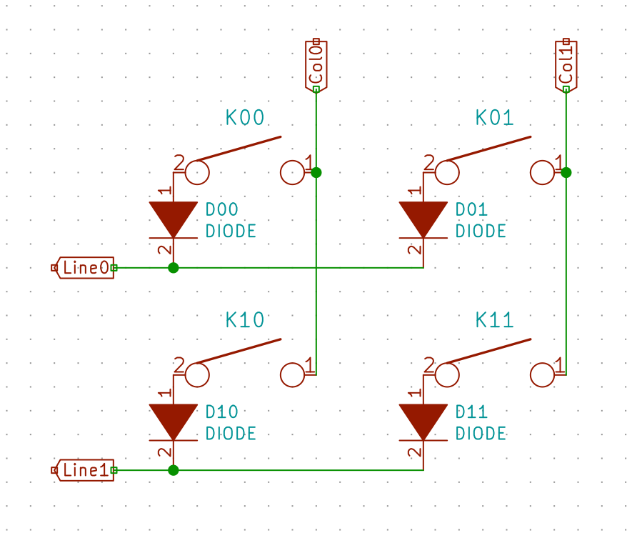
In the same hypothetical scenario as before, the current is prevented to flow back from K00 to K01 and from Line0 by the D01 diode. Thus when powering Col0, the controller will only see a tension on Line0, but not Line1. And when powering Col1 it will see a tension from Line0 and Line1, thus registering 3 key presses, as it should.
That being said, let’s start our work on the electronic schema.
The last time I designed a PCB was during my engineering degree. And it was a long time ago. Things have changed nowadays. We now have open source software to design electronic schemas and PCB, no need to purchase a very expensive EDA software anymore, we have factories to build PCB at very low cost, etc.
Let’s start by installing the PCB design software: Kicad.
Since I was very rusty in this field, I needed a refresher on PCB design and keyboard inner workings. Hopefully, the keyboard community and especially ai03 has hosted a lot of very useful resources. The most important one is ai03’s awesome book on keyboard PCB design.
If you want to also start designing a PCB, I would suggest to read ai03’s tutorial (several times) and try to follow every steps. That’s a good way to get familiar with Kicad and its shortcuts.
One of his first advice is to work on the project under a git repository and to frequently commit. This is by far the most important advice I would recommend. It will allow you to come back in time if you fail something (and bonus point you can push to GitHub or any other central Git repository system to share your design).
So I started by creating a git repository, and added the keyboard kicad libraries I needed as git submodules:
Once done, fire Kicad and choose “File” -> “New Project”, and locate your git repository (make sure to uncheck working in a subdirectory). Kicad will have created 2 files:
.sch file containing the electric schema.kicad_pcb file containing the PCB itselfWe’re going to add our symbols and footprint libraries to the Kicad project.
Go to Preferences -> Manage Symbol Libraries, then add our 3 libraries as explained in this screenshot:
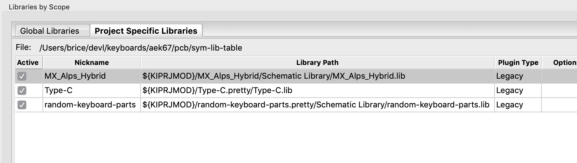
Next, go to Preferences -> Manage Footprint Libraries, and add our 3 footprints libraries (do not pay attention to the 2 extras libraries in my screenshot as I took it in a different project):
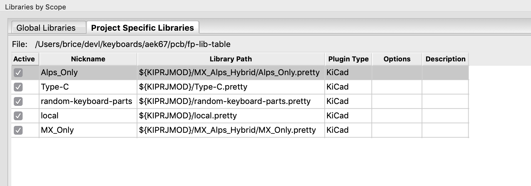
Note how I reference the libraries with the Kicad variable ${KIPRJMOD} which is a shorthand for the project location. This means that the project is relocatable (and anyone can check it out from GitHub without missing symbols problems).
Also note that I created a “local” footprints library in which we can put footprints we might need in this project but that are not in any specific library (or if we don’t want to import the whole library).
So the very first thing is to design the electric schema. In our case the electric schema has 3 distinct parts:
We’re going to use an Atmega32U4 as the MCU. This is the iconic MCU for keyboards, it is inexpensive, very well supported by QMK, has direct USB connectivity, comes with a factory loaded boot-loader and has enough I/O to drive a 65% matrix.
The design will use an USB-C connector and a protection circuit to prevent electro-static discharges to destroy the keyboard electronics.
To start working on the electronic schema, we double click on the .sch file in the Kicad project. This opens a blank page in the eeschema application.
Follow ai03’s guide to setup the schema grid to 50mils or 25mils.
If you work with a trackpad, make sure to check all 3 checkboxes in the Preferences Zoom & Pan section, otherwise using Kicad becomes very counter intuitive.
To properly use the schema editor, you need to first add a given component (shortcut a) and then wire it accordingly to the data-sheet (shortcut w to draw wire, k to stop wire at the mouse position).
Any action can be cancelled by pressing the Esc key.
To copy an element use the shortcut c while the mouse pointer is on a component and move it (it will be very handy for switches). The shortcut g moves with the wire attached. And finally, you have to know the shortcut e to edit any component characteristic (this is very useful), r to rotate and y to flip a component.
I need to introduce here two notions:
GND and +5V symbols, because those are virtually needed everywhere and we don’t want to clutter our schema with such wires.To place a power symbol, just press p and open the ‘power’ submenu, scroll down to either +5V or GND, then click on the schema to place the symbol, use r to rotate it as you want.
By setting the grid to 50mils, the mouse pointer will snap from point grid to point grid. Every component will be laid out on this grid, and IC pins will also be aligned on such a grid. This way you make sure wires will be connected correctly to the pins of the component without having to precisely aim to the pins. If you were to use a smaller grid, you’d do a lot of small misalignment and some pins would end up not connected.
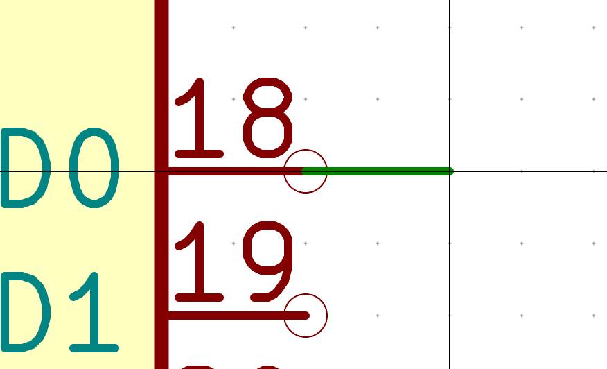
The first thing to do is to add the Atmega32U4 symbol, by pressing the a key, then type Atmega32 in the component search window:
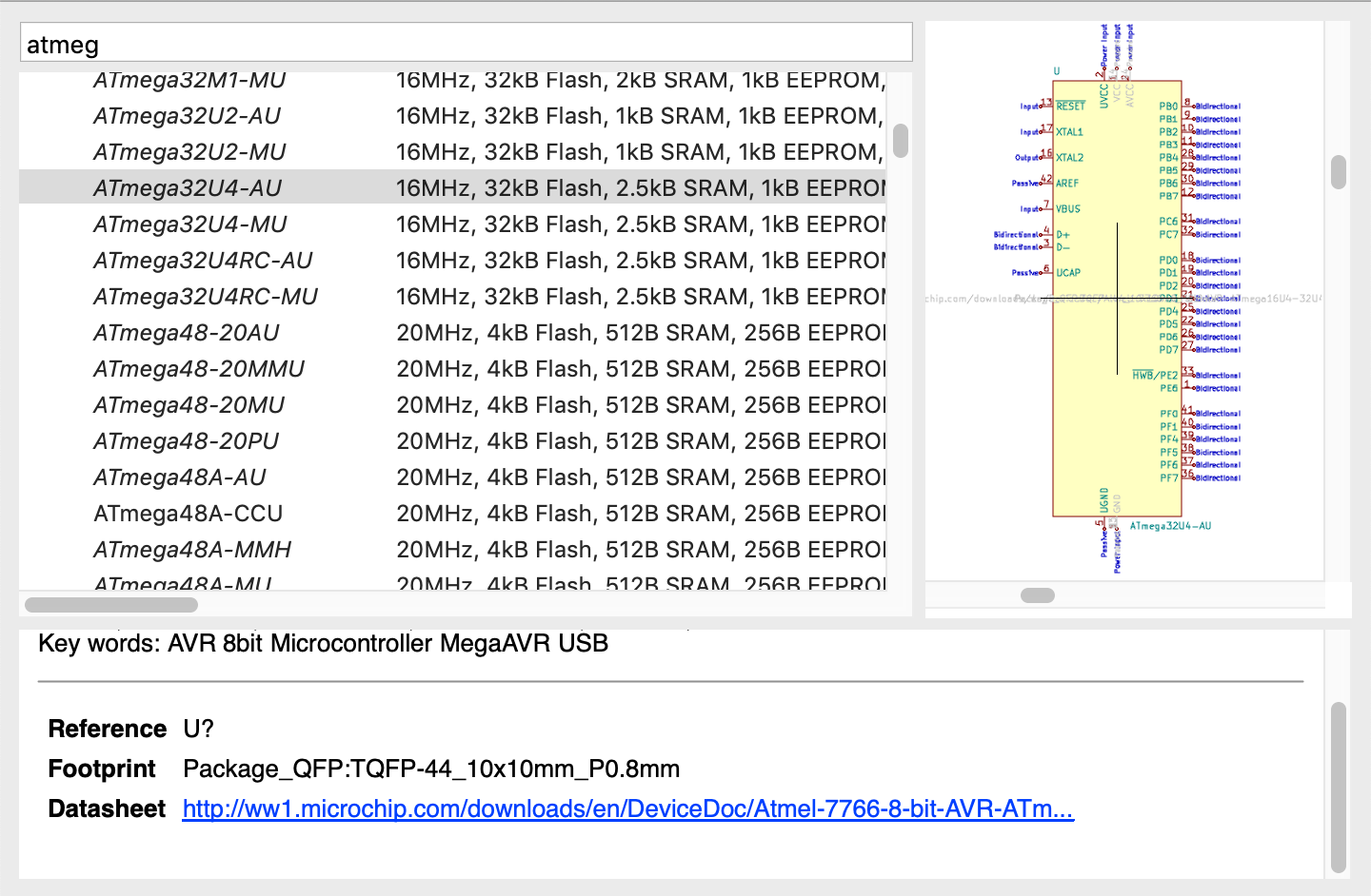
Let’s chose the official Kicad symbol for the Atmega32U4-AU. The AU package is a hand-solderable TQFP format (an IC with apparent pins, unlike the MU variant which is a QFN package where the pins are below making it difficult to solder with a standard solder iron).
Paste the MCU in the grid on the right part of the schema (but anywhere would work).
The MCU is easy to wire, and well explained in ai03’s guide, but to recap:
VCC, AVCC, UVCC should be connected to the +5V power symbol.VBUS should also be connected to the +5V. VBUS is used by the MCU to monitor if it is connected or disconnected to/from the USB port. The Atmega32U4 data-sheets requires it to connect to a 10µF capacitance (see below).GND and UGND should be connected to the GND power symbolThis gives this:
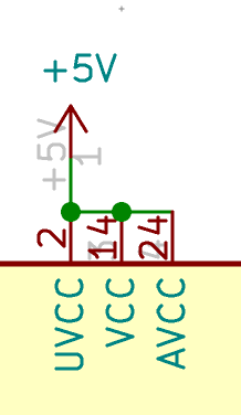
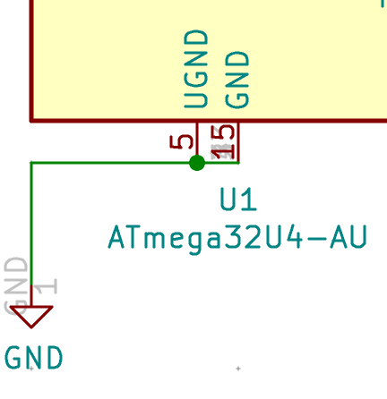
The MCU can work without a clock, but it’s way better to provide it a real external clock. The external clock is a crystal oscillator (or resonator). It is a specific component that produces a square signal at 16 MHz (for our case, otherwise there are crystals for a lot of different frequencies). The MCU is using this clock to sequence instructions execution and other internal functions. When powered with +5V the Atmega32U4 can run at 16 MHz.
For the moment it is enough to add Global Labels to the pins. I’ll cover the crystal circuit a bit later:
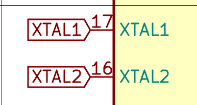
To add a label, press the Ctrl-H key and type it’s name (XTAL1), then place it onto the XTAL1 pin. Do the same with XTAL2. You might need to rotate the label either during creation or afterward (with r).
Let’s do the same with the D+/D- and RESET pins.
The next pin to wire is HWB. HWB is forced to GND with a pull down to make sure the MCU will boot with the boot-loader (refer to the data-sheet for more details). Create a R_small symbol for the resistor (we’ll use R_small symbols for all other resistors), then wire it like this:
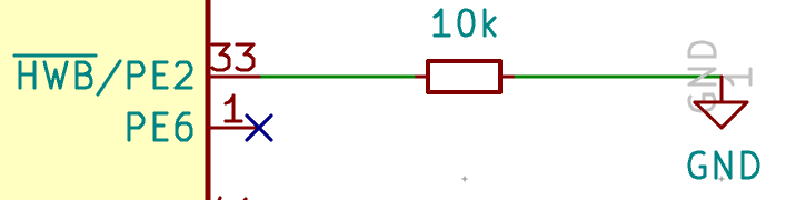
The UCAP is the internal USB pins voltage regulator, it has to be connected to a 1µF capacitor as instructed by the Atmega32U4 data-sheet. Use a C_small symbol for the capacitor (and all capacitors going forward)
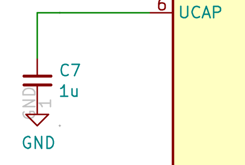
AREF doesn’t need to be wired, we’re going to mark it with a cross by pressing q and clicking on the pin. AREF (and AVCC FWIW) is used when doing analog signaling which we’re not going to do in our keyboard.
The very next step is to design the clock that drives the MCU and which will hook to the XTAL1 and XTAL2 labels.
The Atmega AN2519 tech-note gives a recommended design and equations to compute the capacitance values. Spoiler alert: the capacitor value is 22pF.
Place a Crystal_GND24_small on the grid close to the MCU. Then wire it like this:
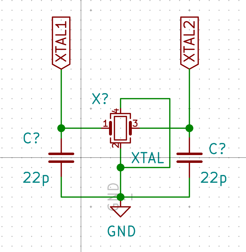
Every component on Kicad has several properties. Among them, we find two important ones:
The reference isn’t attributed when you add a new component to the schema, it contains one or more ?. There is an operation in Kicad that allows to automatically assign references to all the components (we’ll use it soon). This is necessary to be able to create a PCB or run the Electric Design Rule Checker, etc.
To edit the component values and reference, you can press e while hovering the mouse pointer on the symbol. This allows to edit all facets of a given component, including its reference, value, but also it’s symbol and footprint. There are shortcuts to edit the value (v) or the reference (u) directly.
It is possible to move the reference or value label of a component by pressing m while the mouse is over the component. It’s what I did in the crystal schema so that values and references are not colliding with any wires.
The Atmega32U4 data-sheet recommends every +5V pins of the MCU to have decoupling capacitors. The decoupling capacitors play an important role for an active IC. If the component starts to draw current while doing its work, the voltage of the power source will drop, which could be problematic for the component itself but also for all other components powered by the same source (this creates noise on the power line).
To prevent this, we add decoupling capacitors on each power pin of the IC. Those decoupling capacitors will act as local energy storage. When the IC begins to consume energy the capacitors will be able to fulfill it without too much adverse effect on the power source. When the component doesn’t consume energy the decoupling capacitors refills gradually becoming ready for the next serve.
The AN2519 tech notes indicates that every VCC pins of the MCU should be decoupled by a 100nF (or 0.1µF) capacitor.
To be effective, the capacitor must be placed as close as possible from the MCU on the final PCB. Note that there are 4 VCC pins on the Atmega32U4 (2 AVCC, UVCC and 2 x VCC), so ideally we would need 5 100nF capacitor and one 10μF for VBUS. In practice, we can share the 10μF capacitor for both VBUS and UVCC and dispatch the 4 100nF to the other vcc pins.
To prevent cluttering the electronic schema, as ai03 suggests, I’ve placed those decoupling capacitors altogether in the schema.
Start by placing a capacitor, then use the c command to copy and move the next capacitor until you’ve placed all. Then wire them accordingly to this schema:
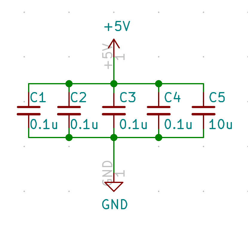
In case of catastrophic failure, it might be necessary to reprogram the Atmega32U4. In this case (for instance if we lost the DFU boot-loader), we can’t use the USB port to do that. We need to access the Serial Peripheral Interface (SPI) programming interface, and use the ISP programming mode.
To do this, we’re going to include on the PCB a 6 pins header with the SPI signals ready:
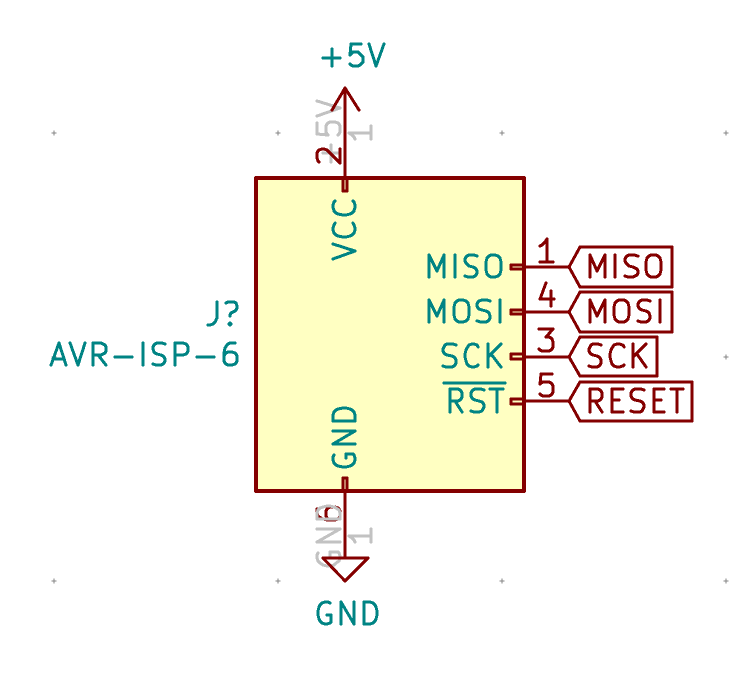
And associate it with the corresponding pins on the MCU:
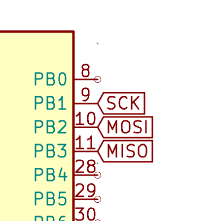
Notice that those 3 signals consume 3 general I/O pins which could be used for connecting the matrix. Since the matrix has 15 rows and 5 lines, it requires 20 I/O pins on the MCU. The MCU has thus enough available I/O pins. However if that wasn’t the case (for instance we might want to dedicate pins to RGB LEDs or backlighting or have a larger matrix), then it is very possible to share the ISP pins with the matrix. During ISP programming those matrix lines won’t be in use and during the keyboard use, the ISP pins won’t be in use. There are alternative matrix configurations to overcome a limited number of pins. Among them, you can double the number of rows and use the same “electrical” column for two consecutive physical columns. Another alternative is called Charlieplexing
The keyboards needs to be flashed with a firmware (we’ll use the ubiquitous and opensource QMK).
The first time the Atmega32U4 boots, it will enter DFU mode because there’s no firmware loaded in the chip. The good thing with those MCU is that it is possible to flash them through the USB port and a program on the computer (for instance QMK Toolbox).
But, once done, if for any reason you need to update the firmware, there’s no way to make the firmware enter the DFU mode anymore (unless you included a RESET key combination in the keymap).
Hopefully, the MCU supports a way to perform an external reset, as the data-sheet explains: “The MCU is reset when a low level is present on the RESET pin for longer than the minimum pulse length.”
That means we can attach a push button to the reset pin to trigger a reset. But the tech notes also states: “The reset line has an internal pull-up resistor, but if the environment is noisy it can be insufficient and reset can therefore occur sporadically”. We don’t want to risk spurious reset, so we also need to add a pull-up resistor.
The AN2519 recommended design is the following one:
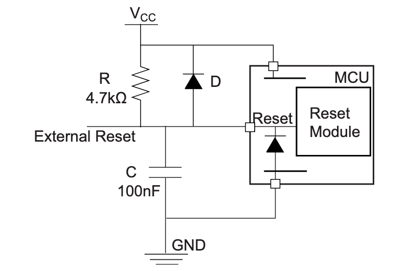
The tech-note recommended design adds a filtering capacitor to prevent noise in very noisy environments. I don’t think this keyboard will be used in such environments, we’re going to skip it (that’s one component less to solder, yay!).
The tech-note next paragraph adds the recommended design for a reset push button (this is to be combined with the):
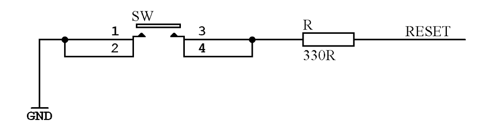
The 330 ohm resistor in series is to prevent a high current to form when shorting the capacitor at the moment the push button is pressed. This in turn would produce a high voltage on the RESET pin of the Atmega32u4 which could destroy it. Since we won’t use the capacitor, we don’t need this resistor altogether.
There’s no need to debounce the push button, because we really don’t care if we ever do multiple resets in a row when it is depressed.
There’s the question of the ESD protection diode parallel to the pull-up resistor. Since we don’t need His-Voltage/Parallel Programming (HVPP) for a keyboard (we’re going to do only USB and ISP flashing), the diode could be needed (otherwise it would prevent getting the 11V-15V needed on the RESET pin to trigger HVPP).
The ESD protection diode is just a standard diode (some recommend a Zener diode there). It protects from any electrostatic discharge damage. During the discharge, the external reset voltage is greater than 5.7V (Vcc 5V + 0.7V for the diode conduction), and the diode then conducts all the current toward the +5V source, thus protecting the RESET pin from the discharge current.
The diode has no interest for ESD protection if we only allow to reset with a push button (our case), but it might be of interest if we allow an external signal to trigger the reset. However the keyboard ISP header is for use only in case of emergency and will be hidden and protected in the keyboard case so the risk of ESD is quite negligible. I think it can be safe to remove this diode from the design.
Most open-source keyboard designs don’t have this diode either, probably for the same reason. To be noted that most of the Atmega32U4-based arduino board out-there don’t have the diode either.
For the real reset button I’m going to use a small SMD button like the RS-187R05A2-DS MT RT or the Alps SKQGAFE010.
The schematic of those buttons shows that there are 4 pins, each pair of pins connected horizontally. There’s no such symbol in Kicad yet. I could use a basic SW_PUSH with the alps footprint for instance and that would work fine. But I can also show you how to create your own symbol.
Let’s open the symbol editor from the Kicad main window. First I’ll create the local library (which has already been added to Kicad earlier). Then in this library, I’m creating the SW_SKQG symbol like this:
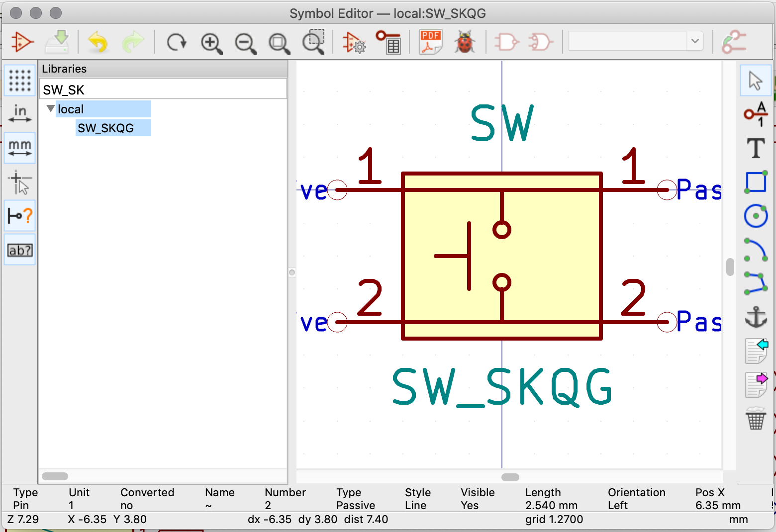
It’s composed of a rectangle, 4 pins labelled 1 & 2 and a few polylines and circles: nothing very complicated. Make sure to keep using the 50 mil grid settings to place the various pins, otherwise it will be difficult to connect the symbol in the schematic. Once done, save the symbol, it is ready to be used in the schematic:
So, finally my reset circuit looks like this:
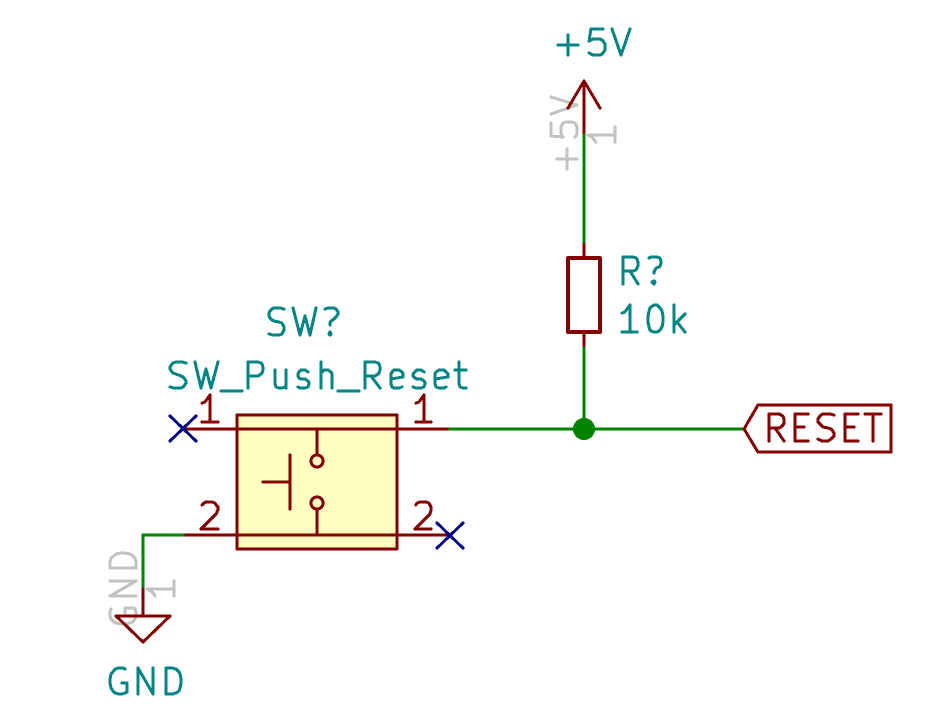
USB Type-C connector are much more usable than Type-B, because they can be reversed. The USB circuit needs to be as protective as possible for the rest of the keyboard electronics as I don’t want the electronic components to be destroyed by an electrostatic discharge (ESD). This means the circuit will have ESD protection on the data lines and power surge protection on the Vcc.
But for ease of building, the USB-C connector must be hand solderable. I had a good experience with the HRO Type-C-31-M-12. It is reasonably cheap, available and easy to hand-solder. Though, the shield contacts don’t completely go through a standard 1.6mm PCB (which is not an issue with metalized holes or thinner PCBs). It’s an USB 2.0 Type-C connector, perfect for a keyboard that doesn’t require hi-speed transfer.
So, let’s add a HRO-TYPE-C-31-M12 component to the schema. It is part of ai03’s Type-C library. An USB-C connector has 2x2 USB 2.0 signal wires, two D+ (DP1 and DP2) and two for D- (respectively DN1 and DN2). The reason there are 2 sets of lines is to provide the reversibility of the connector. We’ll start by connecting those together, with 22 ohms resistors as the Atmega32U4 data-sheet requires:
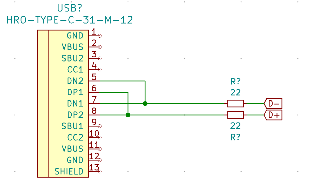
Next, wire both GND and the shield together, then both VBUS pins:
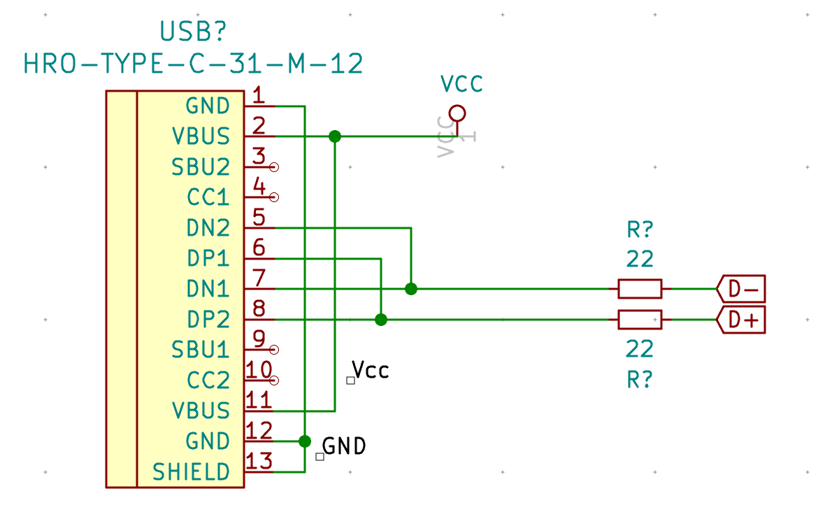
Note that we haven’t declared the +5V signal we’ve used elsewhere in the schema, instead we’ve declared Vcc. We’re going to add a fuse in the next step to protect our +5V against current surge.
Add a Polyfuse_Small to the schema connected to Vcc and +5V likes this:
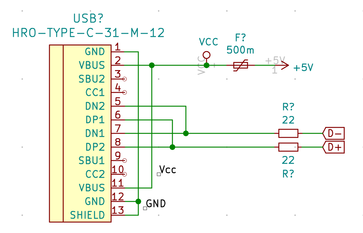
SBU1 and SBU2 are not used (it’s only for Alternate Mode like transporting HDMI or thunberbolt signals), so we can use the ‘No connect flag’ (Shift-Q) to place a black cross on those pins.
Next let’s focus a bit on the CC1 and CC2 pins. Those pins are the Channel Configuration pins. They are used to detect cable attachment and removal detection, plug orientation detection, etc.
The mechanism can be modeled like this:
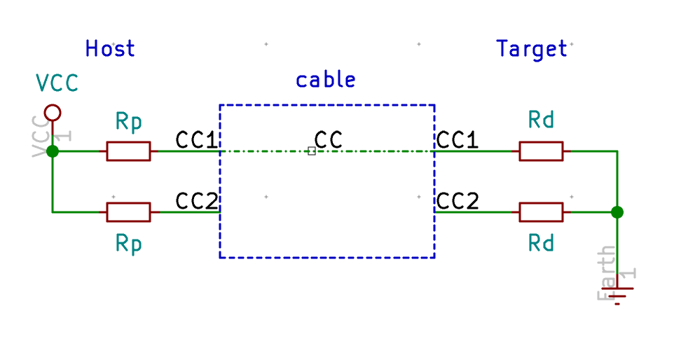
In the above schema we have the host (on the left) connected to the target (our keyboard on the right). Both equipments have pull-up (Rp) or pull-down (Rd) resistors. The USB-C cable has only one connector for CC. In the example above, the host will pull up the level of its CC1 and CC2 pins thanks to the pull-up resistor. The cable connects CC1 on the host to CC1 on the target, creating a current path from the +5V to GND. The host CC1 pin will then have a voltage of less than 5V, while CC2 will still has 5V (no charge). The host then knows the cable is connected (otherwise there would be 5V on both CC1 and CC2) and to which side it is connected to, magic!
Now if we flip the connector at the host for instance, we get the following schema:
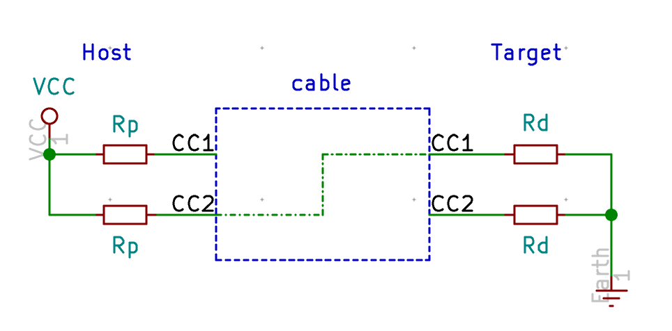
CC2 on the host will see less than 5V but CC1 will see 5V. The host detects it is connected through CC2 and not CC1 as in the previous example.
But there’s more. By choosing properly the value of the Rd resistors we can tell the host, as a target how much current we need to operate. For the USB standard 500mA (which is enough for powering our keyboard), we need 5.1k ohms resistors.
Let’s modify our schema now to add the CC pull-down resistors:
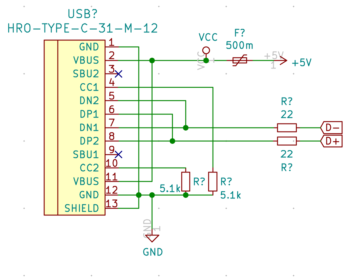
And finally we’re going to add the ESD protection system. We could use rail to rail discrete diodes, but it’s way easier to use an IC. There are several possibilities, one of the simplest is the PRTR5V0U2X. But you might find also the USBLC6 on some designs.
Here’s the modified schema with the PRTR5V0U2X connected to the data lines:

If you followed the design so far, you should have the following schema:
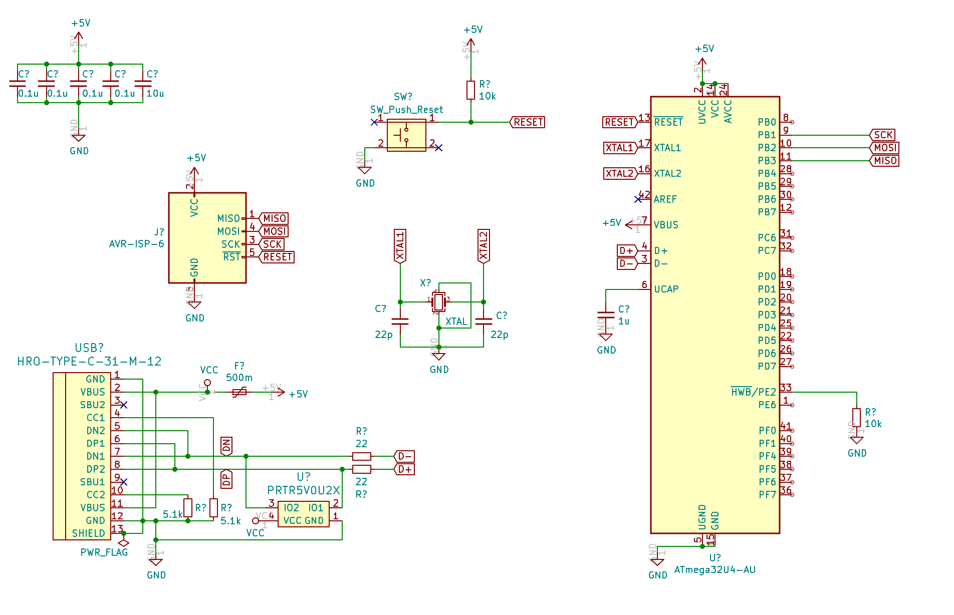
We’re far from having a working PCB. I’m going to cover the following topics in the next episode:
Then on the subsequent parts, I’ll cover soldering SMD components, configuring the firmware, testing the PCB, and designing the case.
Want to read the next part? Then click here for the Designing a Keyboard part 2
In the handwired build log part 1 we saw a technique to build a nice keyboard matrix without using a PCB.
In this part we’ll discover how to hook the teensy controller to the matrix.
For this part, we’ll use:
We’ll also need those parts:
We plan to put the controller on a ribbon cable DIP connector:
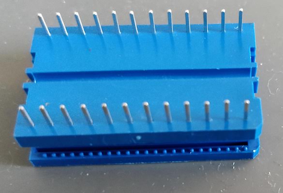
This is a special connector normally used to solder a ribbon cable to a PCB. This connector has the same footprint as a teensy, so instead of soldering it to a PCB, we’ll solder the teensy on the connector.
The ribbon cable will go from this connector to the matrix. To secure the ribbon cable, we need to use some wrench to crimp the connector on the ribbon cable. Each conductor from the ribbon cable ends up on a pin of the DIP connector:
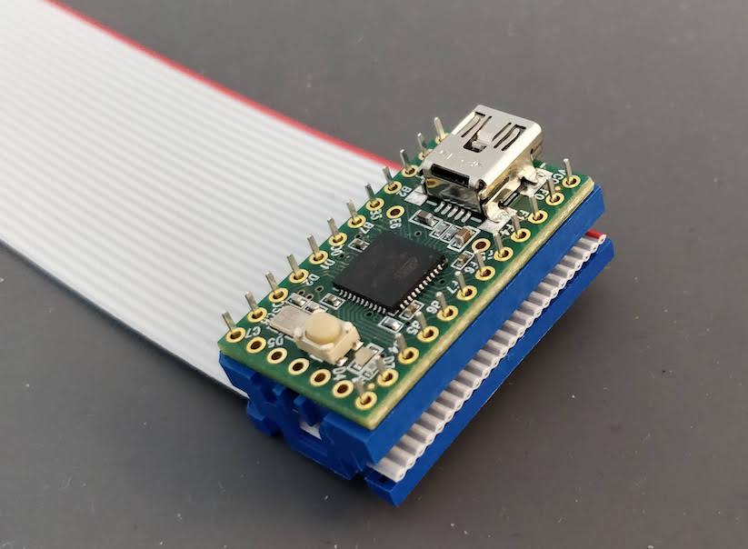
For the controller to read the matrix we need to wire each row and each column to a given port on the MCU. The good thing is that any port will do it, we don’t need to wire specifically a column or a row to a specific port (this would have been different if we had backlight leds which work better with a PWM capable pin).
I didn’t plan any case, but I want in the end to put a transparent PMMA bottom on which I could glue the controller. Since the plate has 5 M2 screw holes, I plan to secure the bottom plate through these holes by using the screws and five PCB brass spacers.
We have 12 columns and 4 rows in the matrix, all those needs to be connected to the MCU ports. That means we’re going to use 16 conductors out of 24 on our ribbon cable.
For aesthetic reasons, and since 12 is a multiple of 4, I’ve splitted the 16 conductors ribbon cable in 4 pieces of 4 conductors.
The idea is to route the 4 conductors ribbon up to where the individual connector will be soldered to the matrix.
The big difficulty is to plan the length of the 4 conductors ribbons and when to split them in individual conductors. Again for aesthetic reasons, I decided to keep the conductors bound together in the ribbon as much as physically possible.
The other good news is that a small ribbon of 4 conductors is about the same size as the distnce between 2 switches. So I can route those ribbons easily under the matrix wires and between the switches up to their respective destinations.
For aesthetic reason again, I decided to route all the ribbons starting from the controller at the same place in the back of the board, and make some 90º turns when needed. So I need to route them sorted by length (ie start by routing the longest ribbon and finish by the smallest one).
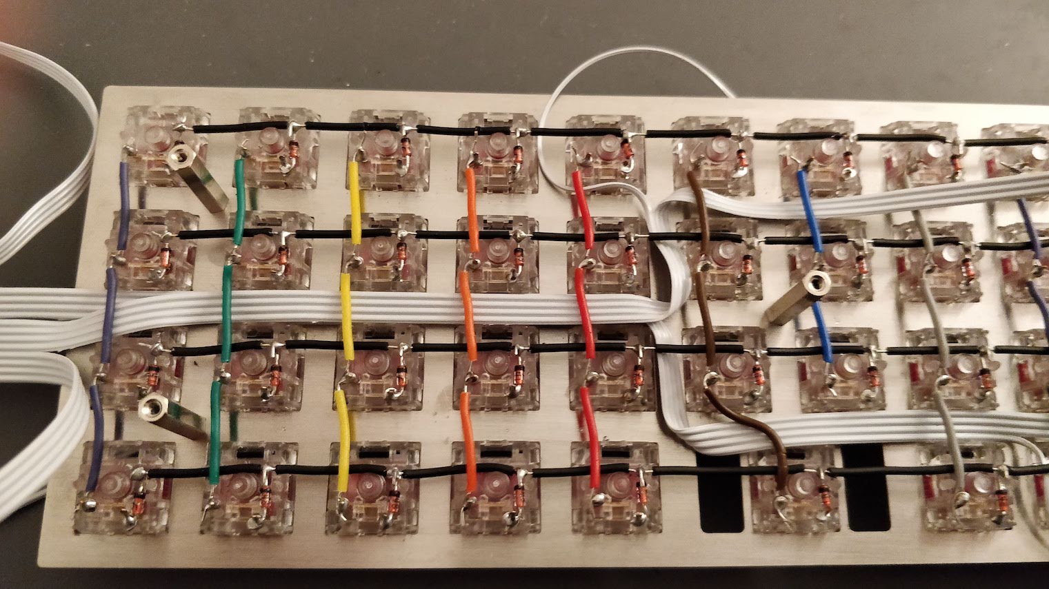
As you can see in the picture, the ribbons turn around the brass spacers. I started routing from the middle lane which was free of spacers until the middle of the plate, then move up or down to access the needed columns.
One thing I didn’t plan very well was that I wanted the controller and its USB port to be on the left of the keyboard. But I did the routing from the left when the keyboard was on the front, so in the end the controller happens to be on the right side. Unfortunately it was to late to change it when I noticed it.
To connect the conductors to the matrix columns, I splitted the ribbon in individual connectors and routed them each to one switch:
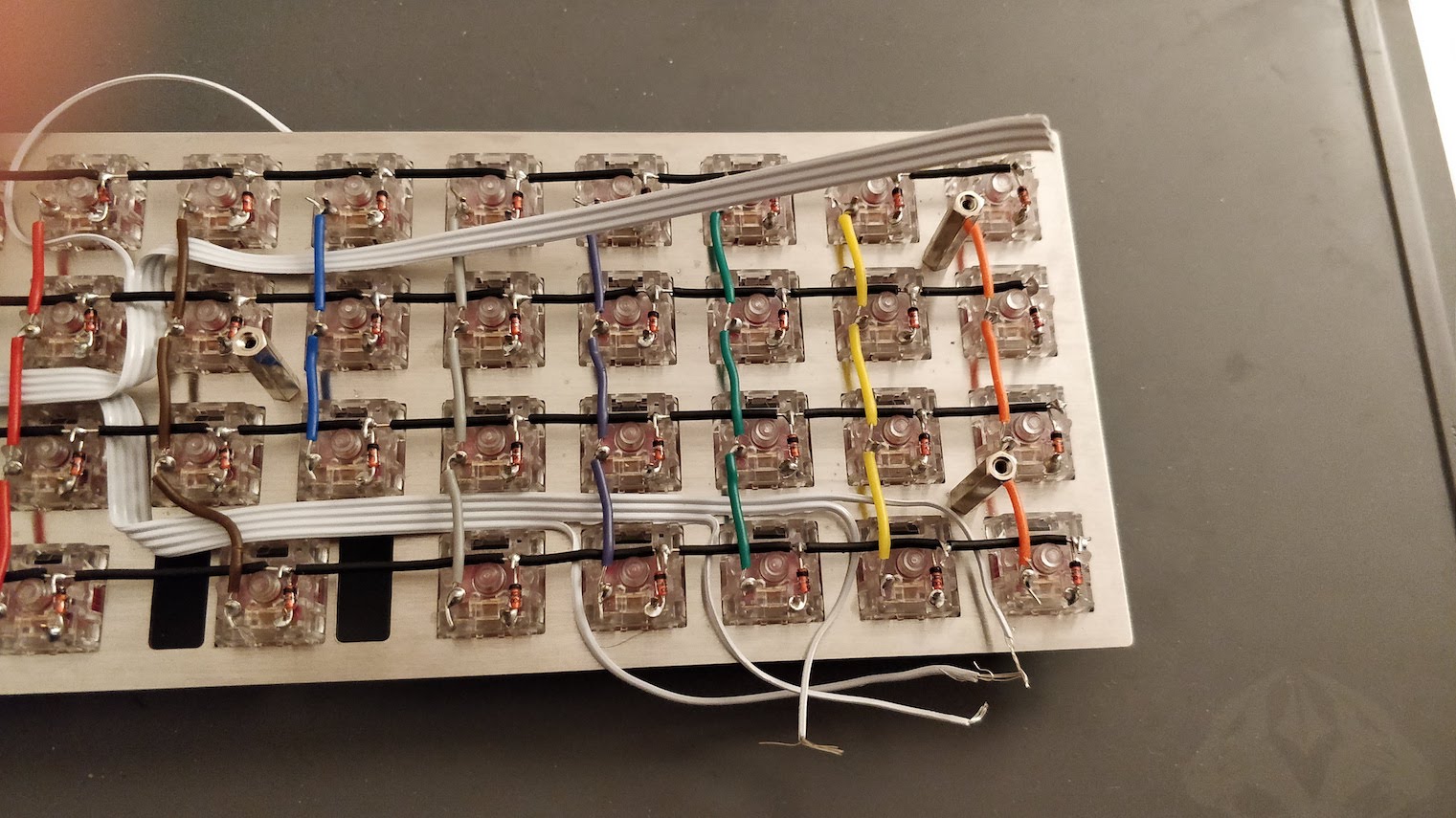
Then it is a matter of cutting the conductor to the right length and remove the insulator. Usually it is not possible to use the wire stripper because it requires a large distance between the cut position and the end of the cable which is not possible when the conductor comes from the plate. I had to remove the insulator using a sharp knife and my nails.
To solder the conductors on the columns, I did a loop with the copper conductors around an existing solder junction, then used the solder iron to heat that existing solder. The loop was incorporated into the existing junction solder easily:
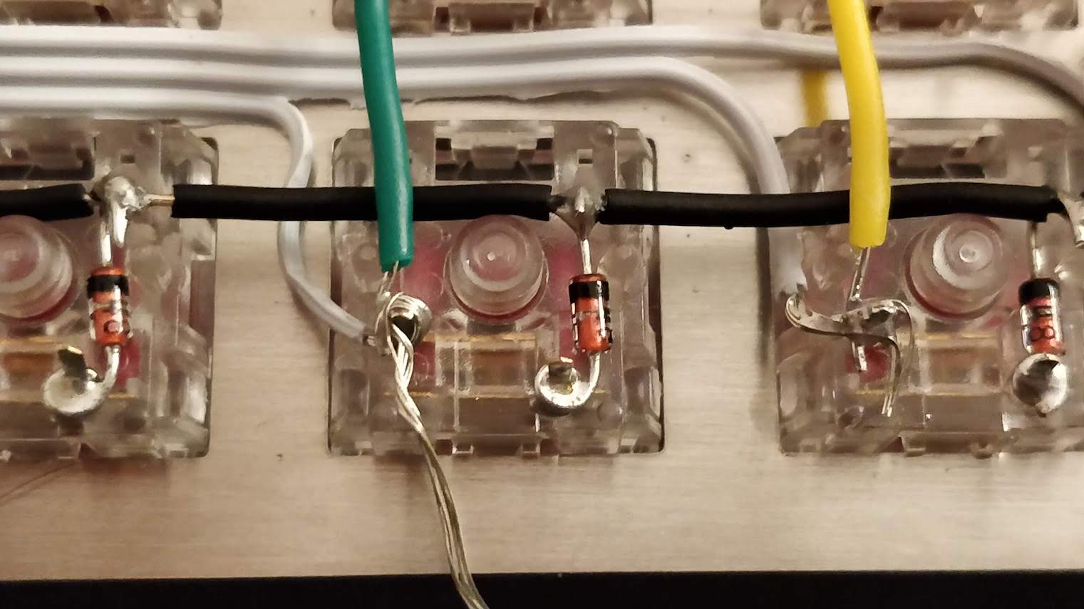
Since we have 12 columns, I decided to route the first 4 conductors ribbon to the column 1 to 4 (the right ones on the back), the second ribbon to the middle ones (5 to 8), and the last column ribbons on the 8 to 12 columns. To balance a bit the routing, the first ribbons connect to the bottom row, the second one to the top row:
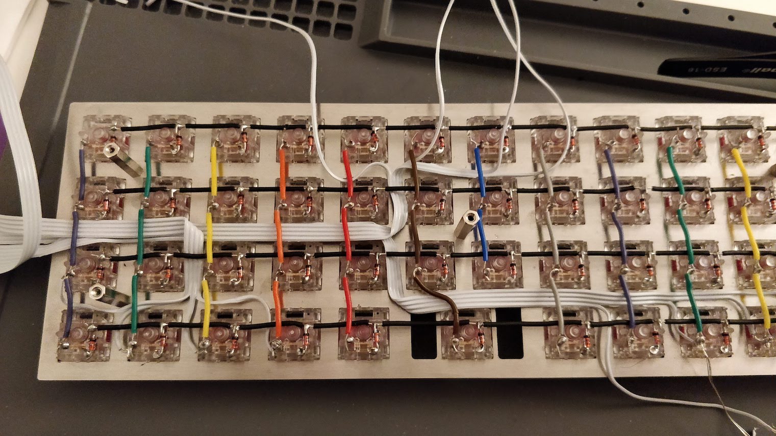
The very next step is to route the last 4 conductors ribbon to the rows. The simples solution was to split the 4 conductors ribbon into 2 parts, one going up and one going down. Then solder the wires to the rows on the same column.
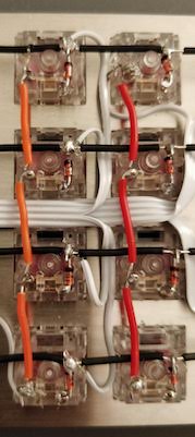
And the final routing result:
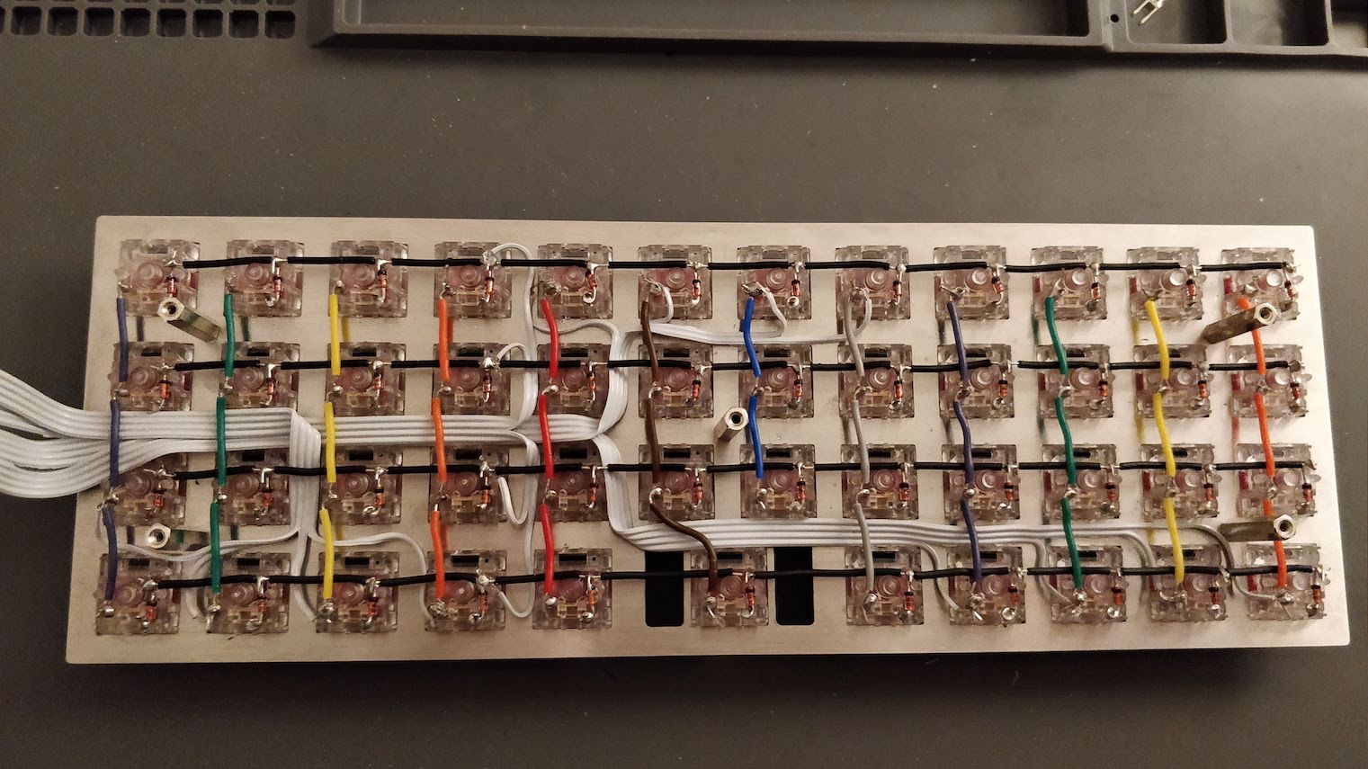
The first step is to crimple the DIP support on the ribbon cable. To help aligning the 16 conductors ribbon, I kept the unused 8 conductors part (this way the ribbon can’t move while closing the support).
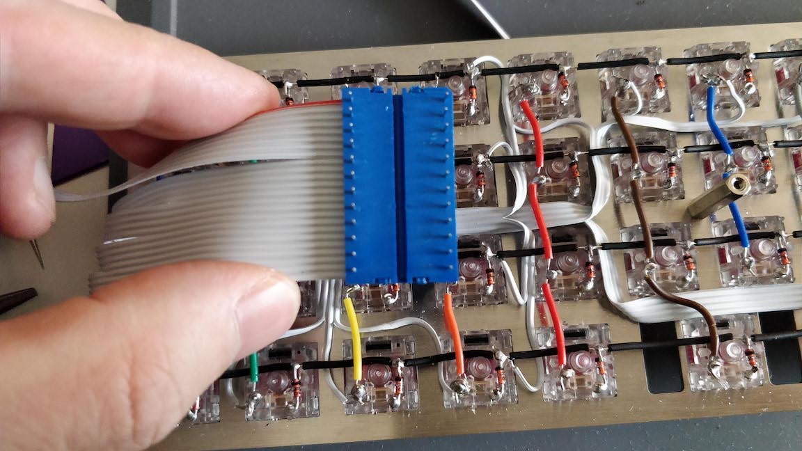
To prevent any electric short between the controller and the switches, the controller is placed upside down, so the support pins are facing down in usual conditions (so the pins are facing up when the keyboard is reversed as in the picture).
Before soldering the controller to the support, I used the multimeter to make sure all the support pins are correctly connected to the matrix. To do that place the black electrode of the multimeter to one of the pin and check it is connected to the correct column or row.
At the same time note which pin is connected to which column or row, as we’ll have to use this information for the firmware:
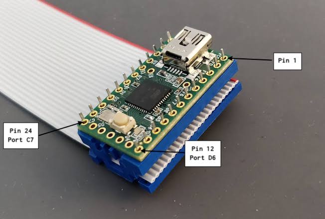
If you follow exactly this tutorial, you’ll end up with this table for the rows:
| row | pin | port |
|---|---|---|
| 1 | 23 | C6 |
| 2 | 11 | D7 |
| 3 | 24 | D7 |
| 4 | 12 | D6 |
And this one for the columns:
| Column | pin | port |
|---|---|---|
| 1 | 19 | D0 |
| 2 | 7 | F7 |
| 3 | 20 | D1 |
| 4 | 8 | B6 |
| 5 | 22 | D3 |
| 6 | 9 | B5 |
| 7 | 21 | D2 |
| 8 | 10 | B4 |
| 9 | 9 | F6 |
| 10 | 18 | B7 |
| 11 | 17 | B3 |
| 12 | 6 | F5 |
Then solder the Teensy controller. It’s not easy as the Teensy PCB pads are very small, so better use a magnifying glass and a very small solder diameter (0.6mm for instance).
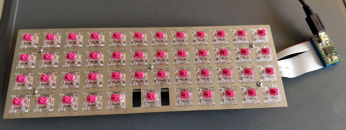
To program the controller we’ll use QMK. This is an open source keyboard firmware forked and enhanced from TMK. It supports a miriad of custom keyboards and MCU (including various ATmega and ARM micro-controllers).
First, let’s clone the project:
git clone git@github.com:qmk/qmk_firmware.git
cd qmk_firmware
Then install the ATmega toolchain to be able to build the firmware for our keyboard. It’s very easy with the install process:
./util/qmk_install.sh
On macos it requires Homebrew.
Once done, check that you can compile a firmware, for instance the default GH60 keymap (a very well known 60% PCB):
% make gh60:default
QMK Firmware 0.6.193
Making gh60 with keymap default

avr-gcc (GCC) 7.3.0
Copyright (C) 2017 Free Software Foundation, Inc.
This is free software; see the source for copying conditions.  There is NO
warranty; not even for MERCHANTABILITY or FITNESS FOR A PARTICULAR PURPOSE.

Compiling: keyboards/gh60/gh60.c                                                                    [OK]
Compiling: keyboards/gh60/keymaps/default/keymap.c                                                  [OK]
Compiling: quantum/quantum.c                                                                        [OK]
Compiling: quantum/keymap_common.c                                                                  [OK]
Compiling: quantum/keycode_config.c                                                                 [OK]
Compiling: quantum/matrix.c                                                                         [OK]
...
Compiling: lib/lufa/LUFA/Drivers/USB/Core/USBTask.c                                                 [OK]
Linking: .build/gh60_default.elf                                                                    [OK]
Creating load file for flashing: .build/gh60_default.hex                                            [OK]
Copying gh60_default.hex to qmk_firmware folder                                                     [OK]
Checking file size of gh60_default.hex                                                              [OK]
 * The firmware size is fine - 16926/28672 (11746 bytes free)
You should obtain the gh60_default.hex file. You can remove it, we won’t use it.
QMK supports many keyboards and many layouts (called keymaps in QMK) for each keyboard. A keyboard is defined by a directory in the keyboards/ folder, and each keymap is also a directory in the keymaps/ folder of a keyboard. To build such keymap, one need to use the make <keyboard>:<keymap> command.
The make command produces a hex file that can be flashed on the controller with QMK Toolbox, which is the recommended method. We can flash from the command line if we know the controller bootloader type, but QMK Toolbox is able to autodetect the correct bootloader, check the file size and so on. QMK Toolbox also acts as a console for the controller allowing to see debug statements.
For the Teensy, we’ll use the “halfkay” bootloader. One advantage of the Teensy compared to the Pro Micro controller (which we could have used), is that the bootloader is very forgiving: for instance a Pro Micro can be bricked if we flash a firmware that is too large for it.
Let’s implement our own Planck layout. The very first step is to create a new kind of keyboard in the handwired/ keyboard folder. Since it is a Planck keyboard, let’s create a planck folder in which we need to add the following files:
keymaps/ folder (in which we’ll create our own default keymap)rules.mk makefile which contains our keyboard definition and QMK features enabledconfig.h which defines how our matrix is connected to the controller portsplanck.c and planck.h which only defines the keymap macro in our caseYou can find all the files in my QMK Handwired Planck branch.
Here’s a condensed version of my config.h:
/* key matrix size */
#define MATRIX_ROWS 4
#define MATRIX_COLS 12

/* Our handwired pin-out */
#define MATRIX_ROW_PINS { C6, D7, C7, D6 }
#define MATRIX_COL_PINS { D0, F7, D1, B6, D3, B5, D2, B4, F6, B7, B3, F5 }
#define UNUSED_PINS { B0, B1, B2, F0, F1, F4, D4, D5, E6 }

/* COL2ROW or ROW2COL */
#define DIODE_DIRECTION COL2ROW
We defined here that the matrix is 4x12, and the ports of the rows and columns (in increasing order). Also, we tell QMK that we hooked the diodes between the columns and the rows.
In rules.mk, we tell QMK everything about the used controller:
# This is a teensy 2.0
BOOTLOADER = halfkay
# running this MCU
MCU = atmega32u4
# Processor frequency.
F_CPU = 16000000
# Target architecture (see library "Board Types" documentation).
ARCH = AVR8
# Input clock frequency.
F_USB = $(F_CPU)
# Interrupt driven control endpoint task(+60)
OPT_DEFS += -DINTERRUPT_CONTROL_ENDPOINT
# Boot Section Size in *bytes*
#   Teensy halfKay   512
OPT_DEFS += -DBOOTLOADER_SIZE=512
# Build Options
BOOTMAGIC_ENABLE = no       # Virtual DIP switch configuration(+1000)
MOUSEKEY_ENABLE = no        # Mouse keys(+4700)
EXTRAKEY_ENABLE = yes       # Audio control and System control(+450)
CONSOLE_ENABLE = yes        # Console for debug(+400)
COMMAND_ENABLE = yes        # Commands for debug and configuration
NKRO_ENABLE = no            # Nkey Rollover
BACKLIGHT_ENABLE = no       # There are no leds
MIDI_ENABLE = no            # No MIDI controls
AUDIO_ENABLE = no           # We don't have audio
UNICODE_ENABLE = no         # Unicode
BLUETOOTH_ENABLE = no       # We don't have BT
RGBLIGHT_ENABLE = no        # We don't have underglow
I then created the default keymap. Since this is a Planck replica, I copied over the default Planck keymap of the MIT (2u space) layout. A keymap is a folder in the keymaps/ folder.
Usually the layout is described in the keymap.c file.
This keymap is a 3 layers keymap (base, raise, lower). The base layer can be either qwerty (the default), colemak or dvorak.
A layer is a 2D array representing the keycode associated with a matrix switch. A keymap is an array of layouts (see the keymaps symbol in the keymap.c), one per layer.
The keyboard can be in only one layer at a time, and can be programmed to switch to a given layer with a key combination as explained below.
Here’s for example the keymap of the base qwerty layer of my Planck handwired keyboard:
const uint16_t PROGMEM keymaps[][MATRIX_ROWS][MATRIX_COLS] = {
/* Qwerty
 * ,-----------------------------------------------------------------------------------.
 * | Tab  |   Q  |   W  |   E  |   R  |   T  |   Y  |   U  |   I  |   O  |   P  | Bksp |
 * |------+------+------+------+------+-------------+------+------+------+------+------|
 * | Esc  |   A  |   S  |   D  |   F  |   G  |   H  |   J  |   K  |   L  |   ;  |  '   |
 * |------+------+------+------+------+------|------+------+------+------+------+------|
 * | Shift|   Z  |   X  |   C  |   V  |   B  |   N  |   M  |   ,  |   .  |   /  |Enter |
 * |------+------+------+------+------+------+------+------+------+------+------+------|
 * | Brite| Ctrl | Alt  | GUI  |Lower |    Space    |Raise | Left | Down |  Up  |Right |
 * `-----------------------------------------------------------------------------------'
 */
[_QWERTY] = LAYOUT_planck_grid(
    KC_TAB,  KC_Q,    KC_W,    KC_E,    KC_R,    KC_T,    KC_Y,    KC_U,    KC_I,    KC_O,    KC_P,    KC_BSPC,
    KC_ESC,  KC_A,    KC_S,    KC_D,    KC_F,    KC_G,    KC_H,    KC_J,    KC_K,    KC_L,    KC_SCLN, KC_QUOT,
    KC_LSFT, KC_Z,    KC_X,    KC_C,    KC_V,    KC_B,    KC_N,    KC_M,    KC_COMM, KC_DOT,  KC_SLSH, KC_ENT ,
    BACKLIT, KC_LCTL, KC_LALT, KC_LGUI, LOWER,   KC_SPC,  KC_SPC,  RAISE,   KC_LEFT, KC_DOWN, KC_UP,   KC_RGHT
),
...
}
This corresponds to this layout:
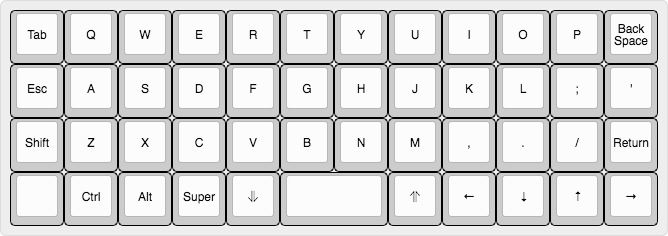
All the people I showed the keyboard asked my why the Esc key is placed below the Tab key. I’m assuming that the original Planck layout has been built this way to enhance the VIM experience. This way the Esc key is on the homerow and can be reached without moving the left hand.
The LAYOUT_planck_grid macro has been defined in our planck.h file. It just maps a keycode to a spot in the layer array representing the matrix.
Notice the two RAISE and LOWER special keycodes. They are layer keycodes defined like this:
#define LOWER MO(_LOWER)
#define RAISE MO(_RAISE)
The MO(layer) macro allows to temporarily activate the given layer when the key is pressed.
The _LOWER and _RAISE layers are defined like this:
...
/* Lower
 * ,-----------------------------------------------------------------------------------.
 * |   ~  |   !  |   @  |   #  |   $  |   %  |   ^  |   &  |   *  |   (  |   )  | Bksp |
 * |------+------+------+------+------+-------------+------+------+------+------+------|
 * | Del  |  F1  |  F2  |  F3  |  F4  |  F5  |  F6  |   _  |   +  |   {  |   }  |  |   |
 * |------+------+------+------+------+------|------+------+------+------+------+------|
 * |      |  F7  |  F8  |  F9  |  F10 |  F11 |  F12 |ISO ~ |ISO | | Home | End  |      |
 * |------+------+------+------+------+------+------+------+------+------+------+------|
 * |      |      |      |      |      |             |      | Next | Vol- | Vol+ | Play |
 * `-----------------------------------------------------------------------------------'
 */
[_LOWER] = LAYOUT_planck_grid(
    KC_TILD, KC_EXLM, KC_AT,   KC_HASH, KC_DLR,  KC_PERC, KC_CIRC, KC_AMPR,    KC_ASTR,    KC_LPRN, KC_RPRN, KC_BSPC,
    KC_DEL,  KC_F1,   KC_F2,   KC_F3,   KC_F4,   KC_F5,   KC_F6,   KC_UNDS,    KC_PLUS,    KC_LCBR, KC_RCBR, KC_PIPE,
    _______, KC_F7,   KC_F8,   KC_F9,   KC_F10,  KC_F11,  KC_F12,  S(KC_NUHS), S(KC_NUBS), KC_HOME, KC_END,  _______,
    _______, _______, _______, _______, _______, _______, _______, _______,    KC_MNXT,    KC_VOLD, KC_VOLU, KC_MPLY
),

/* Raise
 * ,-----------------------------------------------------------------------------------.
 * |   `  |   1  |   2  |   3  |   4  |   5  |   6  |   7  |   8  |   9  |   0  | Bksp |
 * |------+------+------+------+------+-------------+------+------+------+------+------|
 * | Del  |  F1  |  F2  |  F3  |  F4  |  F5  |  F6  |   -  |   =  |   [  |   ]  |  \   |
 * |------+------+------+------+------+------|------+------+------+------+------+------|
 * |      |  F7  |  F8  |  F9  |  F10 |  F11 |  F12 |ISO # |ISO / |Pg Up |Pg Dn |      |
 * |------+------+------+------+------+------+------+------+------+------+------+------|
 * |      |      |      |      |      |             |      | Next | Vol- | Vol+ | Play |
 * `-----------------------------------------------------------------------------------'
 */
[_RAISE] = LAYOUT_planck_grid(
    KC_GRV,  KC_1,    KC_2,    KC_3,    KC_4,    KC_5,    KC_6,    KC_7,    KC_8,    KC_9,    KC_0,    KC_BSPC,
    KC_DEL,  KC_F1,   KC_F2,   KC_F3,   KC_F4,   KC_F5,   KC_F6,   KC_MINS, KC_EQL,  KC_LBRC, KC_RBRC, KC_BSLS,
    _______, KC_F7,   KC_F8,   KC_F9,   KC_F10,  KC_F11,  KC_F12,  KC_NUHS, KC_NUBS, KC_PGUP, KC_PGDN, _______,
    _______, _______, _______, _______, _______, _______, _______, _______, KC_MNXT, KC_VOLD, KC_VOLU, KC_MPLY
),
...
Since on a 40% keyboard we can’t have access to the numbers, function keys, and most of the symbols, those are placed on a different layer than the regular direct access keys. The two raise/lower keys can be actionned by the left and right thumb while at the same time pressing another key to obtain the number or symbol. This is very efficient.
The _______ is an alias for KC_TRANS which means that this key isn’t defined in this layer. When pressing this key while being in this layer, the keycode that will be emited is the first one to not be KC_TRANS in the layer stack. That means that Enter for instance is still Enter in any of the RAISE or LOWER layer.
The rest of the keymap.c file contain special code that overrides the default QMK behavior.
In QMK, a keyboard can override some functionalities, and a keymap can override the keyboard override.
For instance we overrode the process_record function by defining the process_record_user function in our keymap. This is a function which is called each time a key event happens (a key pressed or released). In our case, this is used to switch to a different base layer when going to the ADJUST layer and pressing a base layer key (for instance it is K to switch to colemak). The ADJUST layer is obtained by pressing at the same time the LOWER and RAISE keys.
We also overrode layer_state_set_user to make the LOWER + RAISE = ADJUST layer switching work. The layer_state_set_user function is called whenever QMK is switching to another layer, giving a chance to modify the target layer. We used update_tri_layer_state to return ADJUST when we switched to both LOWER and RAISE.
Now let’s build our firmware:
% make handwired/planck:default
QMK Firmware 0.6.193
Making handwired/planck with keymap default

avr-gcc (GCC) 7.3.0
Copyright (C) 2017 Free Software Foundation, Inc.
This is free software; see the source for copying conditions.  There is NO
warranty; not even for MERCHANTABILITY or FITNESS FOR A PARTICULAR PURPOSE.

Compiling: keyboards/handwired/planck/planck.c                                                      [OK]
Compiling: keyboards/handwired/planck/keymaps/default/keymap.c                                      [OK]
Compiling: quantum/quantum.c                                                                        [OK]
Compiling: quantum/keymap_common.c                                                                  [OK]
Compiling: quantum/keycode_config.c                                                                 [OK]
Compiling: quantum/matrix.c                                                                         [OK]
Compiling: tmk_core/common/host.c                                                                   [OK]
Compiling: tmk_core/common/keyboard.c                                                               [OK]
Compiling: tmk_core/common/action.c                                                                 [OK]
Compiling: tmk_core/common/action_tapping.c                                                         [OK]
Compiling: tmk_core/common/action_macro.c                                                           [OK]
Compiling: tmk_core/common/action_layer.c                                                           [OK]
Compiling: tmk_core/common/action_util.c                                                            [OK]
Compiling: tmk_core/common/print.c                                                                  [OK]
Compiling: tmk_core/common/debug.c                                                                  [OK]
Compiling: tmk_core/common/util.c                                                                   [OK]
Compiling: tmk_core/common/eeconfig.c                                                               [OK]
Compiling: tmk_core/common/report.c                                                                 [OK]
Compiling: tmk_core/common/avr/suspend.c                                                            [OK]
Compiling: tmk_core/common/avr/timer.c                                                              [OK]
Compiling: tmk_core/common/avr/bootloader.c                                                         [OK]
Assembling: tmk_core/common/avr/xprintf.S                                                           [OK]
Compiling: tmk_core/common/magic.c                                                                  [OK]
Compiling: tmk_core/common/command.c                                                                [OK]
Compiling: tmk_core/protocol/lufa/lufa.c                                                            [OK]
Compiling: tmk_core/protocol/usb_descriptor.c                                                       [OK]
Compiling: tmk_core/protocol/lufa/outputselect.c                                                    [OK]
Compiling: lib/lufa/LUFA/Drivers/USB/Class/Common/HIDParser.c                                       [OK]
Compiling: lib/lufa/LUFA/Drivers/USB/Core/AVR8/Device_AVR8.c                                        [OK]
Compiling: lib/lufa/LUFA/Drivers/USB/Core/AVR8/EndpointStream_AVR8.c                                [OK]
Compiling: lib/lufa/LUFA/Drivers/USB/Core/AVR8/Endpoint_AVR8.c                                      [OK]
Compiling: lib/lufa/LUFA/Drivers/USB/Core/AVR8/Host_AVR8.c                                          [OK]
Compiling: lib/lufa/LUFA/Drivers/USB/Core/AVR8/PipeStream_AVR8.c                                    [OK]
Compiling: lib/lufa/LUFA/Drivers/USB/Core/AVR8/Pipe_AVR8.c                                          [OK]
Compiling: lib/lufa/LUFA/Drivers/USB/Core/AVR8/USBController_AVR8.c                                 [OK]
Compiling: lib/lufa/LUFA/Drivers/USB/Core/AVR8/USBInterrupt_AVR8.c                                  [OK]
Compiling: lib/lufa/LUFA/Drivers/USB/Core/ConfigDescriptors.c                                       [OK]
Compiling: lib/lufa/LUFA/Drivers/USB/Core/DeviceStandardReq.c                                       [OK]
Compiling: lib/lufa/LUFA/Drivers/USB/Core/Events.c                                                  [OK]
Compiling: lib/lufa/LUFA/Drivers/USB/Core/HostStandardReq.c                                         [OK]
Compiling: lib/lufa/LUFA/Drivers/USB/Core/USBTask.c                                                 [OK]
Linking: .build/handwired_planck_default.elf                                                        [OK]
Creating load file for flashing: .build/handwired_planck_default.hex                                [OK]
Copying handwired_planck_default.hex to qmk_firmware folder                                         [OK]
Checking file size of handwired_planck_default.hex                                                  [OK]
 * The firmware size is fine - 17618/32256 (14638 bytes free)
Our firmware is in the handwired_planck_default.hex file.
To flash it:
*** Halfkay device connectedATMega32U4 microcontrollerYou should see something like this:
*** Halfkay device connected
*** Attempting to flash, please don't remove device
>>> teensy_loader_cli -mmcu=atmega32u4 /Users/brice/devl/qmk_firmware/handwired_planck_default.hex -v
    Teensy Loader, Command Line, Version 2.1
    Read "handwired_planck_default.hex": 17618 bytes, 54.6% usage
    Found HalfKay Bootloader
    Programming..........................................................................................................................................
    Booting
*** Halfkay device disconnected
*** masterzen - Planck connected -- 0xFEED:0x6060
At this point your computer should recognize that a new keyboard has been connected. If you press any switches it should produce a letter.
You can now test the keyboard and the keymap with the Keyboard Tester.
It can be hard to find nice 40% ortho keycaps. I used the MDA Big Bang set. It’s a nice, smooth (and not that expensive) thick PBT keyset with dye-sub legends that covers a wide range of ortholinear keyboards, including the Planck.
The MDA (also called MIX or EDRUG) profile is a newer key profile that we could call the little brother of the SA profile. It’s less sculpted than SA, but still more than the other profiles.
Here’s how it looks on this handwired Planck:
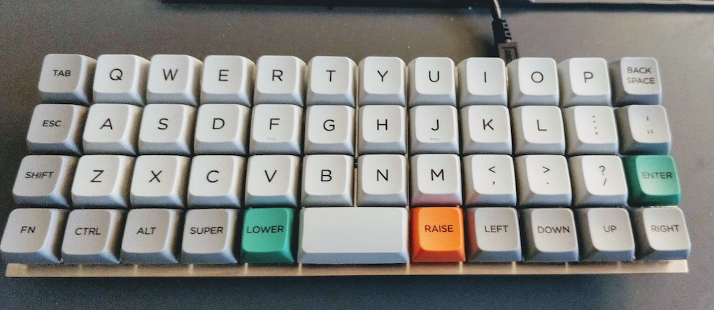
I haven’t had the time to work again on the keyboard, but I want to make it a bit slimmer (it has currently a height of 2cm not including keycaps and switches), and add a transparent bottom plate with small rubber feets.
I plan the bottom plate to be a transparent plexiglass plate (so that we can see the matrix), cut at the size of the metal switch plate. The complex part will be to correctly align the holes for the brass spacer screws along with making sure the hole head fits inside the plate.
To reduce the keyboard height, I will have to carve a small part of the bottom plate so that a small part of the teensy height can fit inside.
If possible, I’d like to build a full case made of plexiglass. I need to design it properly and find the correct tools to do that.
This will probably be the part 3 of this series!
Update 1: I’ve finished the second part of the serie
Update 2: The plate I’m using has a height of 1.5mm, not 2.5mm as some astute readers have pointed out.
For the last 7 months, I’ve been discovering a new hobby: DIY mechanical keyboards. I’ve been using mechanical keyboards for ages (I was mostly typing on a Code keyboards lately), but lately moved to type only on my macbook keyboard (hopefully this is an early 2015, so the keyboard ie bearable).
So 7 months ago, I was browsing the Internet when I discovered a new world: there were passionate people that are building their keyboards and even programming them with QMK.
I soon was embarked in a no return journey to find the perfect keyboard, made of custom keyboards purchased from Korean Group Buys, properly prepared keyboard switches, custom color keycaps, split backspace layouts…
Forward to a month ago, I discovered that some people were building their own keyboards without any PCB, I then decided to try following the best handwiring guide with one of the smallest existing keyboard.
This serie of posts is the story behind this keyboard:
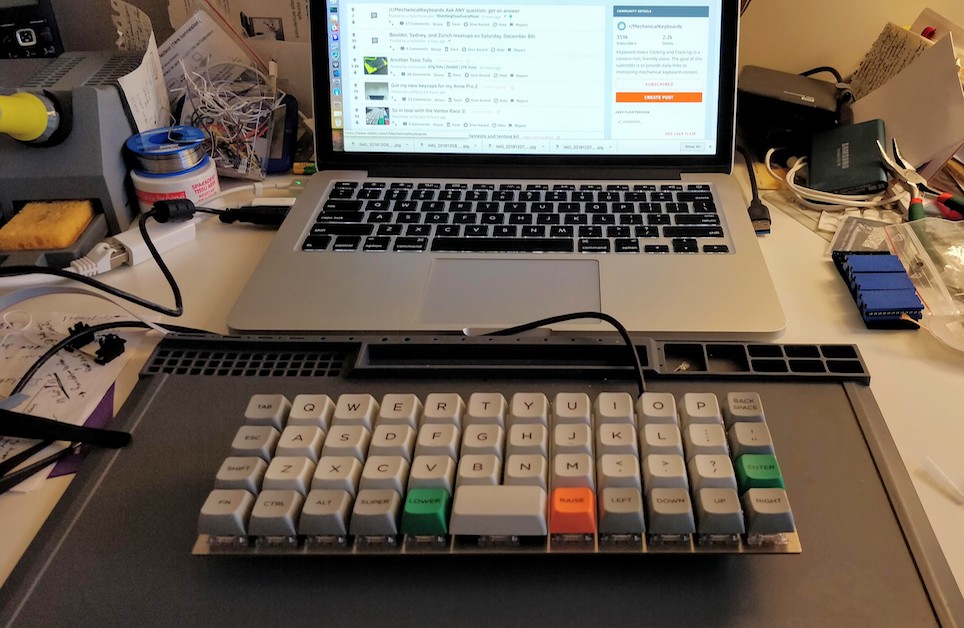
A keyboard if the combination of the following elements:
So in a very fast loop, the controller’s firmware will power on one column of the matrix and “read” the tension back on the matrix rows. If there’s some tension on one row given current on a column, then the controller can deduce which switch has been pressed. The firmware will then send the corresponding keycode based on the layout to the USB port, and continue with the next column and so on infinitely.
But there’s a problem: if one presses more than one key at a time, it is possible for the controller to register ghost keypresses. See the following schema:
When the controller will power the Col0, and if K00, K01 and K11 are depressed simultaneously, the controller will read current on both Line0 and Line1, because the current will flow from Col0 to K00 pin 1, then pin 2 because the switch is depressed, then to switch K01, then to switch K11, then to Line1. For the controller it is as if all the switches have been pressed, instead of the 3 that were indeed depressed.
To prevent this we add diodes between the switch and the row it is connected to:
In the same hypothetical scenario as before, the current will be prevented to flow back from K00 to K01 and from Line0 by the D01 diode. Thus when powering Col0, the controller will only see a tension on Line0. And when powering Col1 it will see a tension from Line0 and Line1, thus registering 3 key presses.
Handwiring as its name implies is an electronic technique of building electronic circuits without using a PCB, and instead wiring all components one by one manually with small electric wires. It is often used to perform prototype of electronic boards.
The aim of this build log is to show how to wire a fully working (but small) keyboard.
We’re going to build a Planck like keyboard in MIT layout, that is a matrix of 4x12, with a 2u spacebar, accounting for 47 keys. I chose this keyboard and layout because it’s one of the smaller keyboard (a 40%) and it is ortholinear (all switches are aligned) making it easy to wire.
So what will we need to build our keyboard:
The MIT layout Planck plate looks like this:
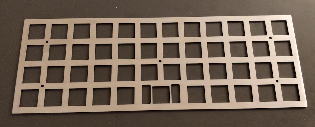
Note that this plate has holes for a PCB mount stabilizer for the 2u space bar. I should have taken a version for a plate mount stabilizer, because with a PCB we won’t be able to put a stabilizer under the space bar.
We’ll also need the following tools:
The most important part is the insulator stripper:

You can get a Vise Grip or any other tool like this one. You might need to tune it’s strength (there’s usually a small knob on the tool) so that it doesn’t cut the small wires.
In this part of the story, we’ll only need the wire stripper, some colored wires, the plate, 47 switches, tweezers, a multimeter, the wire cutter, solder and the soldering station.
The very first step of our handwiring work is to firmly clips the switches on the plate:
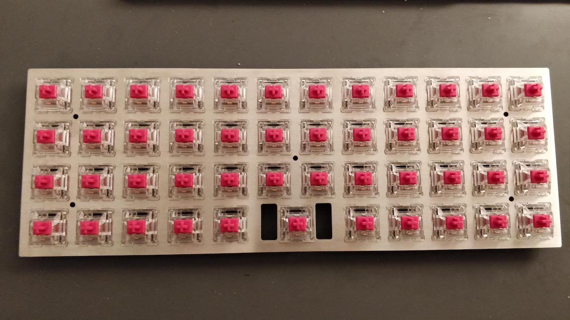
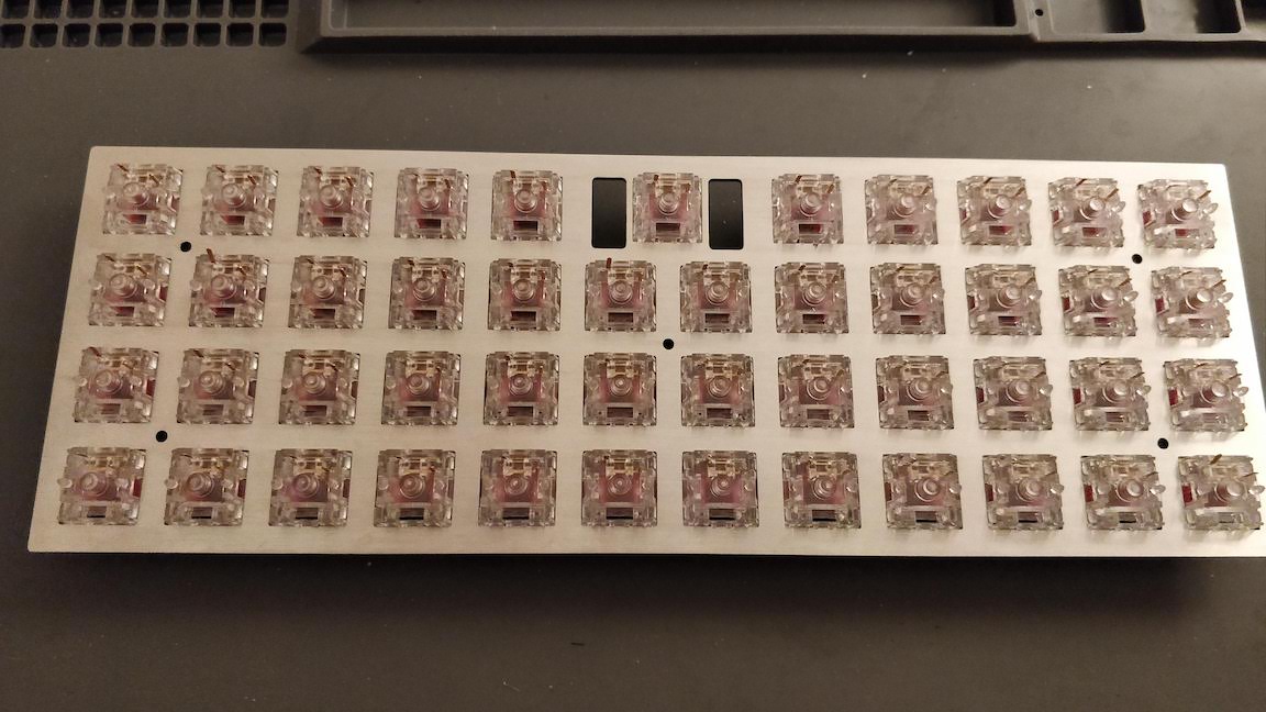
I put the switches facing north (the led hole is at the top) so that the higher pins when seen from the back of the plate will be the pin connected to the rows, and the other one will be connected to the columns.
With a 2.5mm plate, the switches should clipse correctly on it. Make sure the plate is using MX switch holes without “top-opening” punches (straight square holes).
We’ll have to solder the diodes on the switch pin connected to a row. Since there’s no circuit copper pads to put the solder on like on a PCB, the best way to solder something on a pin is to form a small wire loop and put solder on it. The solder will “flow” between the pin and the loop and stick firmly.
So our first task is to form a small loop with one of the leg of the diodes. Make sure to do it on the correct leg: the one opposite to the diode black mark:
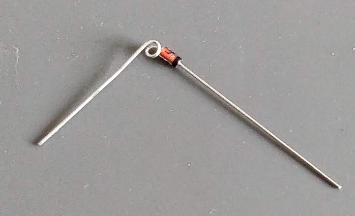
To ease the process and especially if you got your diodes in bands, you can bend them all in one shot on your desk table like this:
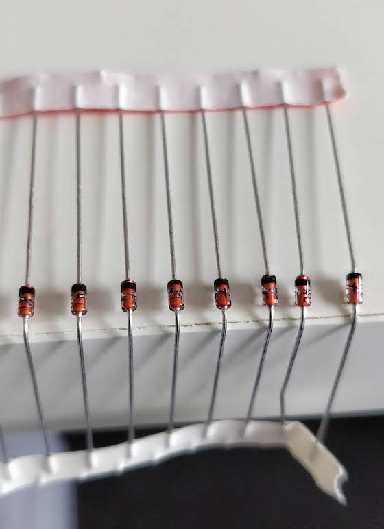
Next, remove the diodes from the strip, and using a tweezer block the wire in it and form a loop by turning around the diode leg. With the tweezer you can make sure the loop is flat. Make sure the loop is big enough to be placed on a switch pin, if not open it a little bit with the tweezers.
Repeat this for the other 46 diodes.
After this you can cut the extraneous diode leg just after the loop:
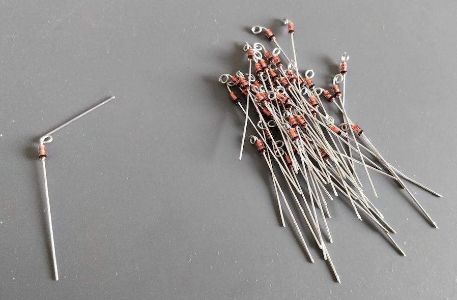
The very next step is to place the diode loops on each of the switch row pins:
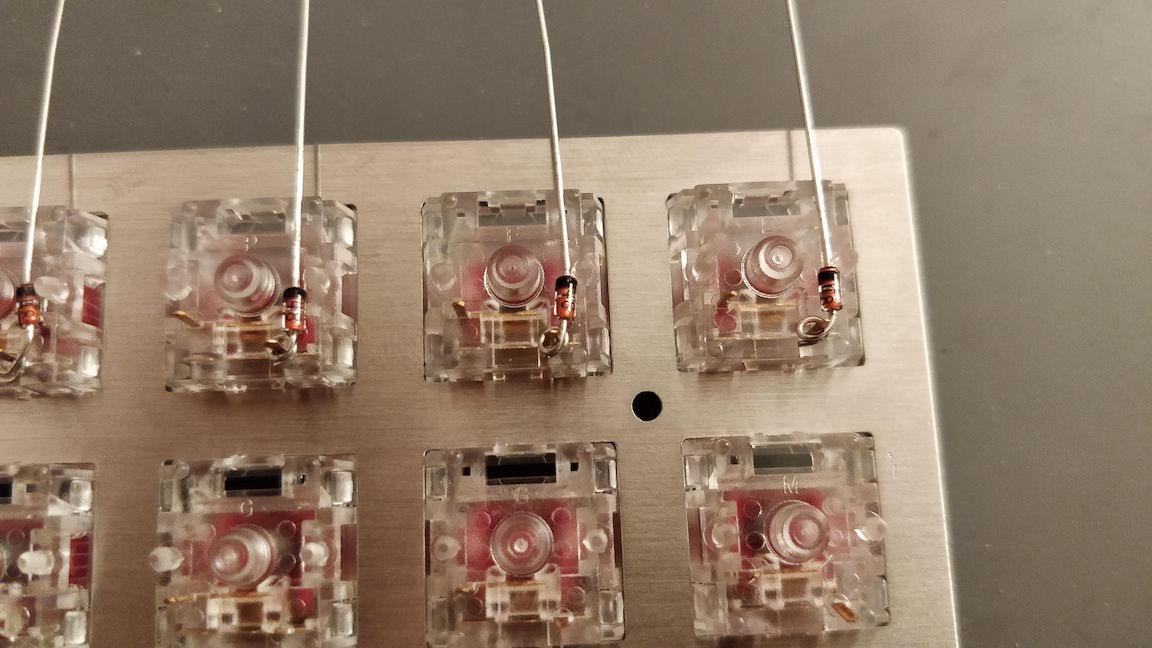
And then soldering them:
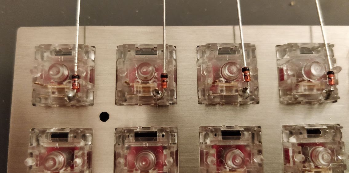
Make sure to orient correctly the diodes and leave the other leg correctly aligned.
Notice that I started placing and soldering the diodes from the top row (as seen from the back) so that the other rows diodes long legs doesn’t hinder soldering the next row.
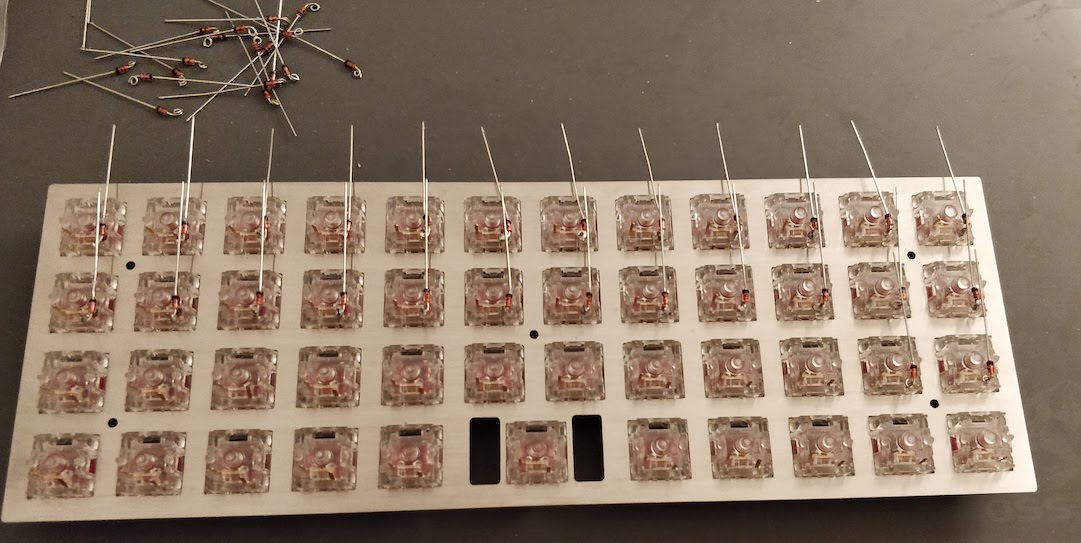
We’ll then keep adding diodes and soldering them until we’ve covered all switches:
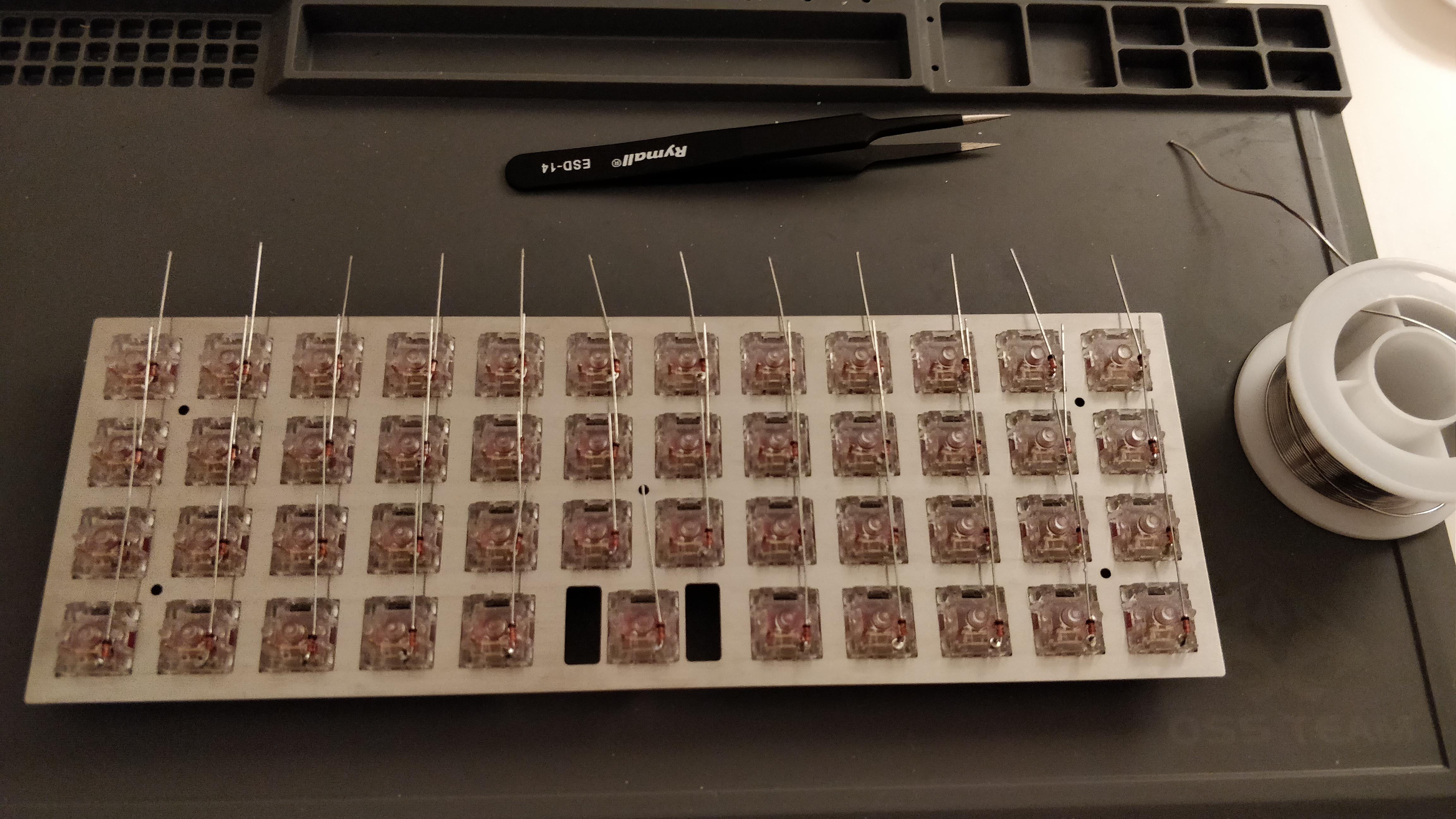
It is important to not cut the remaining leg yet. We’ll use it to connect to the row wire as you’ll find in the next step.
To build the rows, we’ll take a long piece of wire (I used black wire). The first thing to do is to remove the insulator at the loose end on something like 5cm with the wire stripper.
We know that we have 12 switches on a row (except the bottom one which has only 11 switches). There is 19mm between two switches.
Instead of cutting 11 pieces of wire which will be hard to solder in place correctly, we’ll use only one long straight piece of wire on which we’ll split the insulator with the wire stripper into 11 pieces of around 16mm each (without cutting the cable). Since it is hard to correctly measure the insulator length while using the wire stripper, I used a visual clue on the wire stripper to approximate the correct length and aligned the insulator pieces with it before cutting.
To solder the wire, we’re going to bend the diode leg around the cable to form a half loop and solder between the insulator pieces. At the same time secure the row wire with the switch central bumps.
We’ll start by soldering the loose end on the first diode, then proceed to the next diode: push the insulator piece toward the first junction, solder and move back the insulator at equal distance:
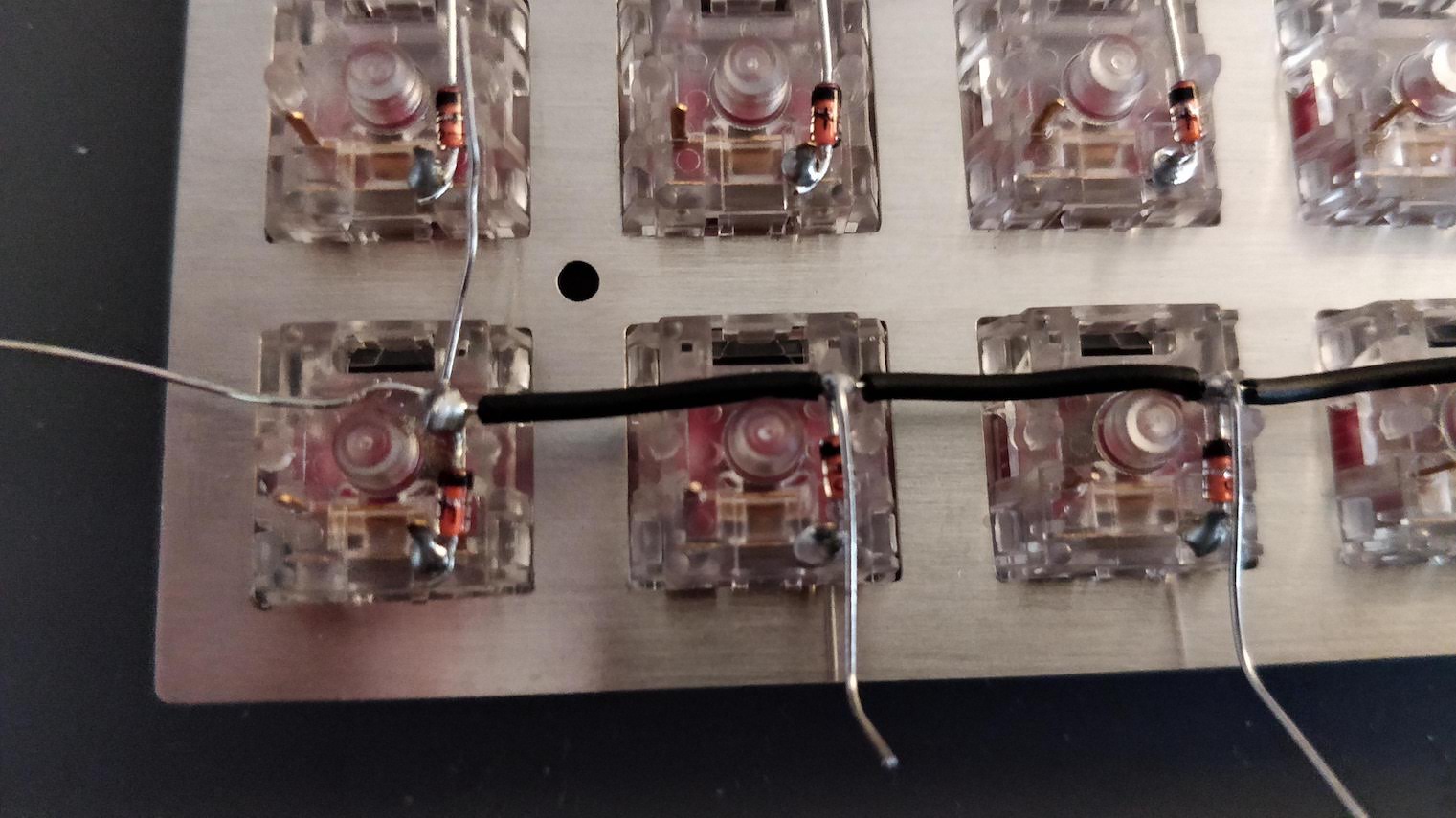
For the first diode, I formed a complete loop with the leg around the wire. For the subsequent diode since it is not practical to do that, I’ve done only half loops.
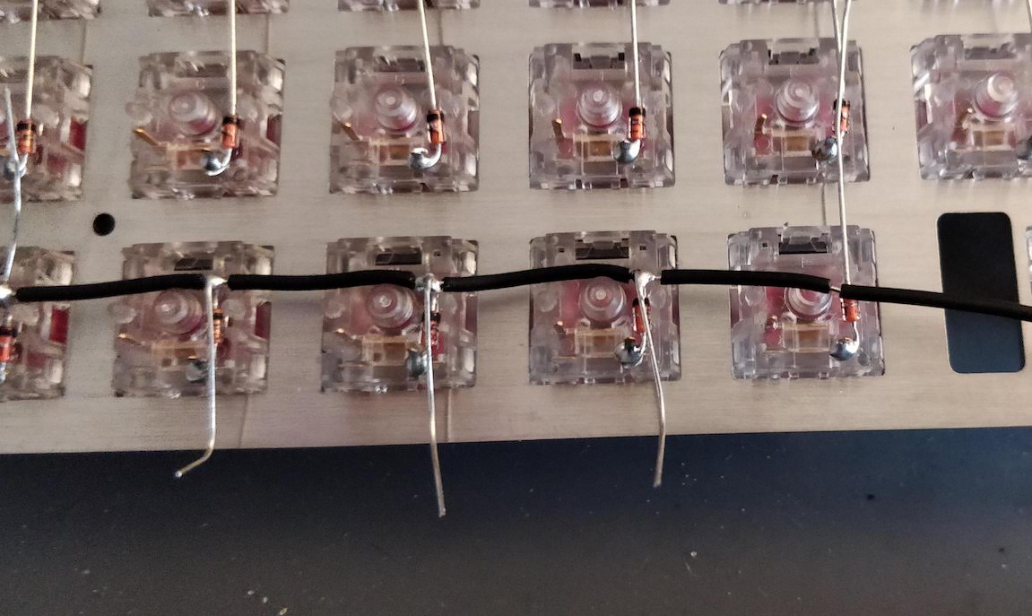
Another option which I used at first is to cut the insulator with the wire stripper on each step instead of cutting the 11 pieces at once. So solder one diode leg, cut the insulator at the right lenght, push it toward the last soldered diode, solder the next one, and so on. This is more effective if the distance between switches is variable, otherwise use the first method.
The last diode in the row should also be soldered by forming a full loop with the diode leg around the wire.
It is important to solder the diode leg on the wire before moving to the next diode leg along the row, otherwise the cable could move during the process and nothing would be correctly aligned.
Cut the extraneous wire at both ends and all the remaining legs with the wire cutter and you should obtain something like this:
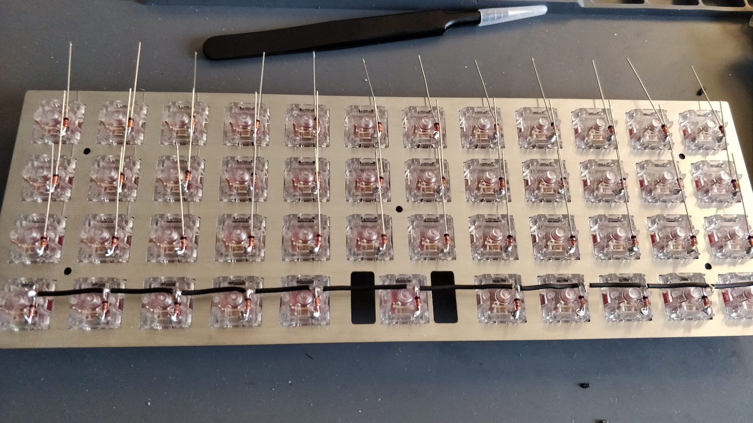
Apply the same technique to the 3 remaining rows. It takes around 10 minutes to solder a 12 switches row:
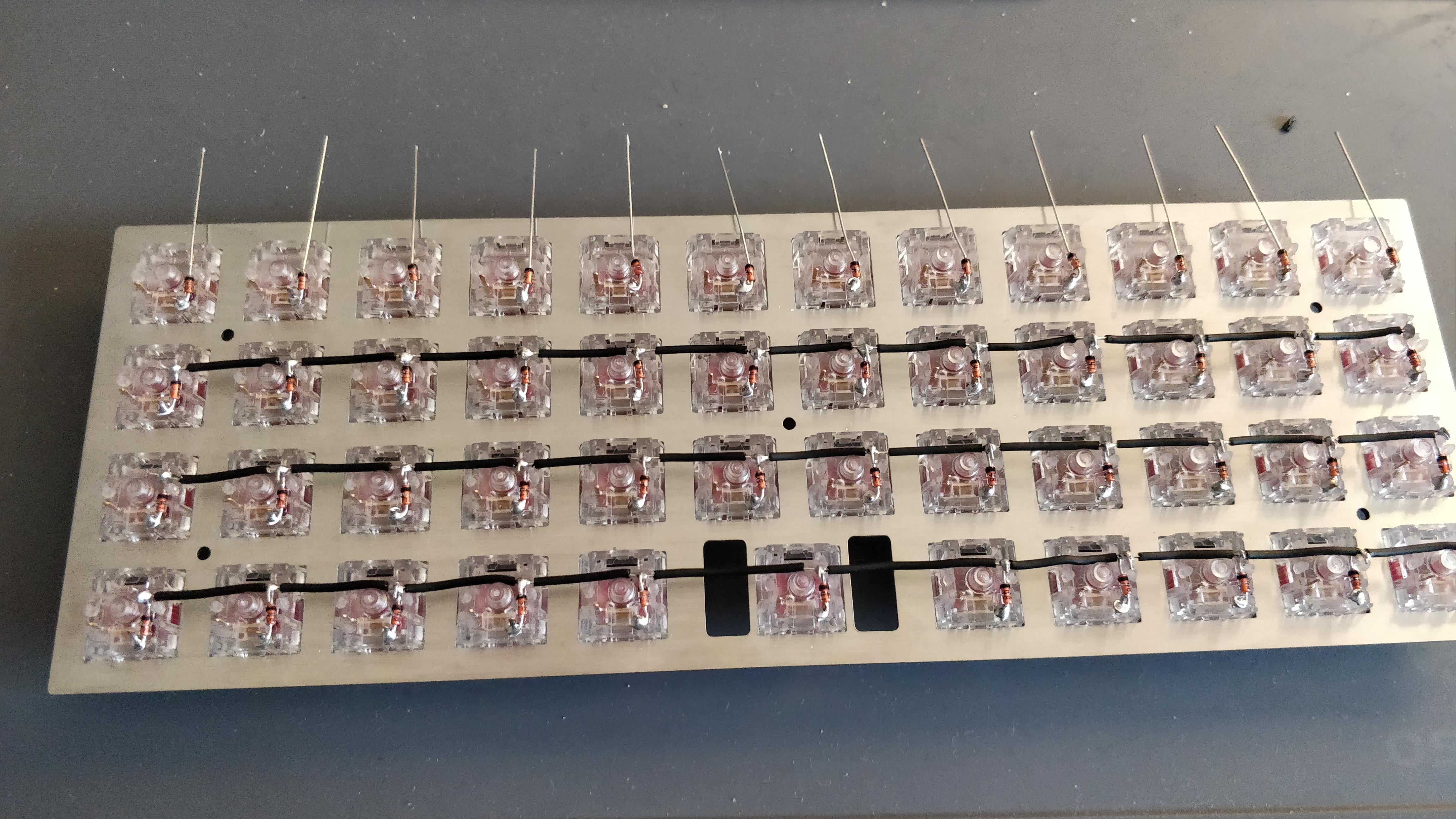
At this stage, you can check with a multimeter that each switch is correctly connected to the wire. Use the multimeter in continuity mode (the multimeter will beep if there is continuity between two junctions), and put the black electrode on one row end and place the red one on every diode junction, there should be a beep. You can also test the continuity of the switches and diodes combination: still with the black electrode on the row, place the red one on the other switch pin and press the switch: the multimeter should beep.
Once you’ve made sure everything works electrically, it is time to move to the columns wiring.
For a better visual effect, I’ve decided to wire each column with a different wire color. Unfortunately I couldn’t find 12 different wire colors, so I’ve used only 6 that I repeated twice. I arranged the colors in an approximation of a rainbow.
We’ll use the exact same technique as for the rows, except that we need to split the insulator into only 3 pieces of equal length (there are only 4 rows on this keyboard). To make sure we have enough wire, I didn’t cut it before soldering the last switch in a column.
Since we don’t have the diodes leg to form a loop around the wire, we’ll build loops with the wire around the switch pins:
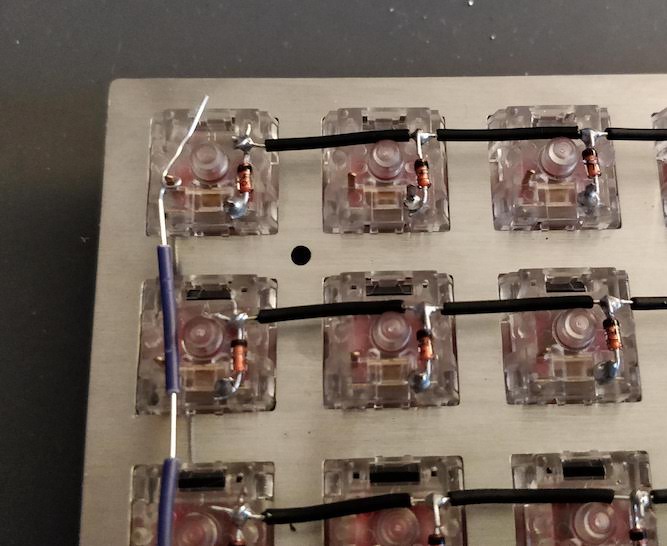
Once soldered we can move to the next switch, push back the insulator toward the previous switch, solder the current one and so on:
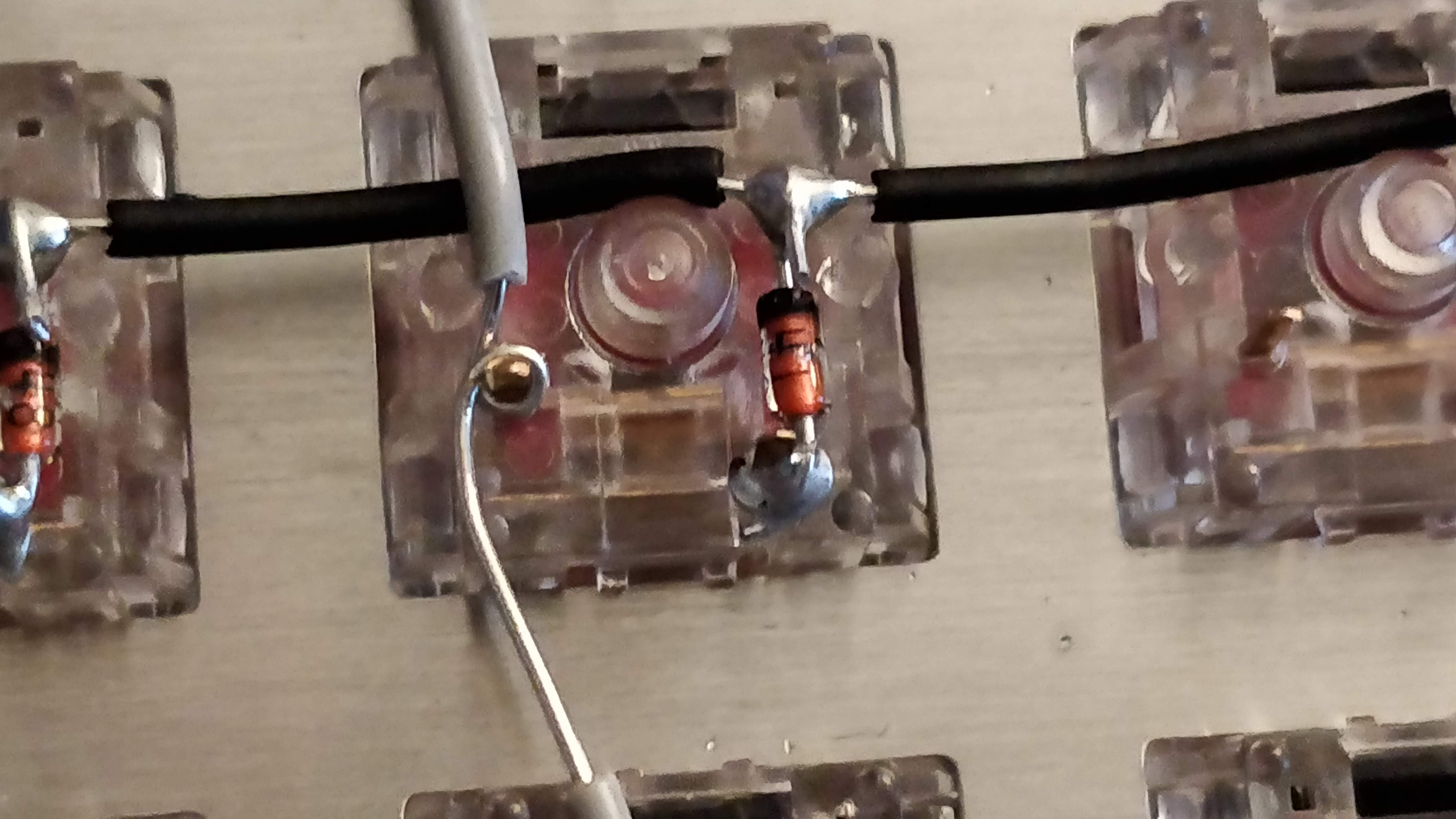
Keep doing this until you’ve done all columns. It takes only a few minute per columns once we get the habit.
Since there are only 11 switches on the bottom row, one of the column will span only 3 switches.
The result should look like this:
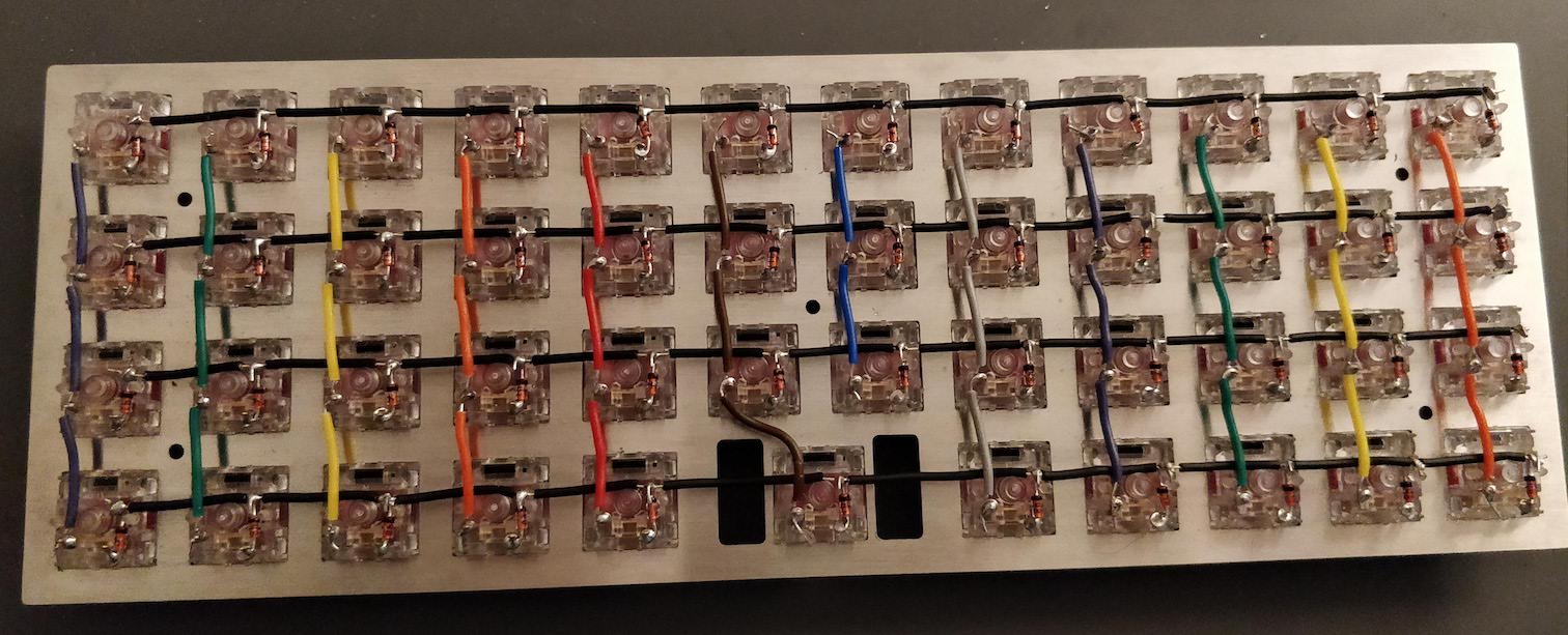
You can then use the multimeter to check the colums are correctly wired, and that no rows is electrically connected to a column.
In the handwired build log part 2, I’ll explain how to connect the controller to the matrix and how to program the controller to become a working keyboard. We’ll also put some keycaps on.
Another part will explain how I’m going to build a bottom plate for the keyboard.
All started a handful of months ago, when it appeared that we’d need to build some of our native software on Windows. Before that time, all our desktop software at Days of Wonder was mostly cross-platform java code that could be cross-compiled on Linux. Unfortunately, we badly needed a Windows build machine.
In this blog post, I’ll tell you the whole story from my zero knowledge of Windows administration to an almost fully automatized Windows build machine image construction.
But, first let’s digress a bit to explain in which context we operate our builds.
Our CI system is built around Jenkins, with a specific twist. We run the Jenkins master on our own infrastructure and our build slaves on AWS EC2. The reason behind this choice is out of the scope of this article (but you can still ask me, I’ll happily answer).
So, we’re using the Jenkins EC2 plugin, and a revamped by your servitor Jenkins S3 Plugin. We produce somewhat large binary artifacts when building our client software, and the bandwidth between EC2 and our master is not that great (and expensive), so using the aforementioned patch I contributed, we host all our artifacts into S3, fully managed by our out-of-aws Jenkins master.
The problem I faced when starting to explore the intricate world of Windows in relation with Jenkins slave, is that we wanted to keep the Linux model we had: on-demand slave spawned by the master when scheduling a build. Unfortunately the current state of the Jenkins EC2 plugin only supports Linux slave.
The EC2 plugin for Linux slave works like this:
java -jar slave.jar.
The stdin and stdout of the slave.jar process is then connected to the jenkins master through an ssh tunnel.I needed to replicate this behavior. In the Windows world, ssh is inexistent. You can find some native implementation (like FreeSSHd or some other commercial ones), but all that options weren’t easy to implement, or simply non-working.
In the Windows world, remote process execution is achieved through the Windows Remote Management which is called WinRM for short. WinRM is an implementation of the WSMAN specifications. It allows to access the Windows Management Instrumentation to get access to hardware counters (ala SNMP or IPMI for the unix world).
One component of WinRM is WinRS: Windows Remote Shell. This is the part that allows to run remote commands. Recent Windows version (at least since Server 2003) are shipped with WinRM installed (but not started by default).
WinRM is an HTTP/SOAP based protocol. By default, the payload is encrypted if the protocol is used in a Domain Controller environment (in this case, it uses Kerberos), which will not be our case on EC2.
Digging, further, I found two client implementations:
I started integrating Overthere into the ec2-plugin but encountered several incompatibilities, most notably Overthere was using a more recent dependency on some libraries than jenkins itself.
I finally decided to create my own WinRM client implementation and released Windows support for the EC2 plugin. This hasn’t been merged upstream, and should still be considered experimental.
We’re using this version of the plugin for about a couple of month and it works, but to be honest WinRM doesn’t seem to be as stable as ssh would be. There are times the slave is unable to start correctly because WinRM abruptly stops working (especially shortly after the machine boots).
So all is great, we know how to execute commands remotely from Jenkins. But that’s not enough for our sysadmin needs. Especially we need to be able to create a Windows AMI that contains all our software to build our own applications.
Since I’m a long time Puppet user (which you certainly noticed if you read this blog in the past), using Puppet to configure our Windows build slave was the only possiblity. So we need to run Puppet on a Windows base AMI, then create an AMI from there that will be used for our build slaves. And if we can make this process repeatable and automatic that’d be wonderful.
In the Linux world, this task is usually devoted to tools like Packer or Veewee (which BTW supports provisioning Windows machines). Unfortunately Packer which is written in Go doesn’t yet support Windows, and Veewee doesn’t support EC2.
That’s the reason I ported the small implementation I wrote for the Jenkins EC2 plugin to a WinRM Go library. This was the perfect pet project to learn a new language :)
So, starting with all those tools, we’re ready to start our project. But there’s a caveat: WinRM is not enabled by default on Windows. So before automating anything we need to create a Windows base AMI that would have the necessary tools to further allow automating installation of our build tools.
There’s a service running on the AWS Windows AMI called EC2config that does the following at the first boot:
On first and subsequent boot, it also does:
One thing that is problematic with Windows on EC2 is that the Administrator password is unfortunately defined randomly at the first boot. That means to further do things on the machine (usually using remote desktop to administer it) you need to first know it by asking AWS (with the command-line you can do: aws ec2 get-password-data).
Next, we might also want to set a custom password instead of this dynamic one. We might also want to enable WinRM and install several utilities that will help us later.
To do that we can inject specific AMI user-data at the first boot of the Windows base AMI. Those user-data can contain one or more cmd.exe or Powershell scripts that will get executed at boot.
I created this Windows bootstrap Gist (actually I forked and edited the part I needed) to prepare the slave.
First, we’ll create a Windows security group allowing incoming WinRM, SMB and RDP:
aws ec2 create-security-group --group-name "Windows" --description "Remote access to Windows instances"
# WinRM
aws ec2 authorize-security-group-ingress --group-name "Windows" --protocol tcp --port 5985 --cidr <YOURIP>/32
# Incoming SMB/TCP
aws ec2 authorize-security-group-ingress --group-name "Windows" --protocol tcp --port 445 --cidr <YOURIP>/32
# RDP
aws ec2 authorize-security-group-ingress --group-name "Windows" --protocol tcp --port 3389 --cidr <YOURIP>/32
Now, let’s start our base image with the following user-data (let’s put it into userdata.txt):
<powershell>
Set-ExecutionPolicy Unrestricted
icm $executioncontext.InvokeCommand.NewScriptBlock((New-Object Net.WebClient).DownloadString('https://gist.github.com/masterzen/6714787/raw')) -ArgumentList "VerySecret"
</powershell>
This powershell script will download the Windows bootstrap Gist and execute it, passing the desired administrator password.
Next we launch the instance:
aws ec2 run-instances --image-id ami-4524002c --instance-type m1.small --security-groups Windows --key-name <YOURKEY> --user-data "$(cat userdata.txt)"
Unlike what is written in the ec2config documentation, the user-data must not be encoded in Base64.
Note, the first boot can be quite long :)
After that we can connect through WinRM with the “VerySecret” password. To check we’ll use the WinRM Go tool I wrote and talked about above:
./winrm -hostname <publicip> -username Administrator -password VerySecret "ipconfig /all"
We should see the output of the ipconfig command.
Note: in the next winrm command, I’ve omitted the various credentials to increase legibility (a future version of the tool will allow to read a config file, meanwhile we can create an alias).
A few caveats:
System.Net.WebClientwinrm set winrm/config/winrs @{MaxMemoryPerShellMB="1024"}
Unfortunately, this is completely broken in Windows Server 2008 unless you install this Microsoft hotfix
The linked bootstrap code doesn’t install this hotfix, because I’m not sure I can redistribute the file, that’s an exercise left to the reader :)Now that we have our base system with WinRM and Puppet installed by the bootstrap code, we need to create a derived AMI that will become our base image later when we’ll create our different windows machines.
aws ec2 create-image --instance-id <ourid> --name 'windows-2008-base'
For a real world example we might have defragmented and blanked the free space of the root volume before creating the image (on Windows you can use sdelete for this task).
Note that we don’t run the Ec2config sysprep prior to creating the image, which means the first boot of any instances created from this image won’t run the whole boot sequence and our Administrator password will not be reset to a random password.
Now that we have this base image, we can start deriving it to create other images, but this time using Puppet instead of a powershell script. Puppet has been installed on the base image, by virtue of the powershell bootstrap we used as user-data.
First, let’s get rid of the current instance and run a fresh one coming from the new AMI we just created:
aws ec2 run-instances --image-id <newami> --instance-type m1.small --security-groups Windows --key-name <YOURKEY>
We’re going to run Puppet in masterless mode for this project. So we need to upload our set of manifests and modules to the target host.
One way to do this is to connect to the host with SMB over TCP (which our base image supports):
sudo mkdir -p /mnt/win
sudo mount -t cifs -o user="Administrator%VerySecret",uid="$USER",forceuid "//<instance-ip>/C\$/Users/Administrator/AppData/Local/Temp" /mnt/win
Note how we’re using an Administrative Share (the C$ above). On Windows the Administrator user has access to the local drives through Administrative Shares without having to share them as for normal users.
The user-data script we ran in the base image opens the windows firewall to allow inbound SMB over TCP (port 445).
We can then just zip our manifests/modules, send the file over there, and unzip remotely:
zip -q -r /mnt/win/puppet-windows.zip manifests/jenkins-steam.pp modules -x .git
./winrm "7z x -y -oC:\\Users\\Administrator\\AppData\\Local\\Temp\\ C:\\Users\\Administrator\\AppData\\Local\\Temp\\puppet-windows.zip | FIND /V \"ing  \""
And finally, let’s run Puppet there:
./winrm "\"C:\\Program Files (x86)\\Puppet Labs\\Puppet\\bin\\puppet.bat\" apply --debug --modulepath C:\\Users\\Administrator\\AppData\\Local\\Temp\\modules C:\\Users\\Administrator\\AppData\\Local\\Temp\\manifests\\site.pp"
And voila, shortly we’ll have a running instance configured. Now we can create a new image from it and use it as our Windows build slave in the ec2 plugin configuration.
Puppet on Windows is not like your regular Puppet on Unix. Let’s focus on what works or not when running Puppet on Windows.
The obvious ones known to work:
User: Puppet can create/delete/modify local users. The Security Identifier (SID) can’t be set. User names are case-insensitive on Windows. To my knowledge you can’t manage domain users.
Group: Puppet can create/delete/modify local groups. Puppet can’t manage domain groups.
Package: Puppet can install MSI or exe installers present on a local path (you need to specify the source). For a more comprehensive package system, check below the paragraph about Chocolatey.
Service: Puppet can start/stop/enable/disable services. You need to specify the short service name, not the human-reading service name.
Exec: Puppet can run executable (any .exe, .com or .bat). But unlike on Unix, there is no shell so you might need to wrap the commands with cmd /c. Check the Powershell exec provider module for a more comprehensive Exec system on Windows.
Host: works the same as for Unix systems.
Of course that’s expected, mostly because of the used packages. Most of the Forge module for instance are targeting unix systems. Some Forge modules are Windows only, but they tend to cover specific Windows aspects (like registry, Powershell, etc…), still make sure to check those, as they are invaluable in your module Portfolio.
You certainly know that Windows paths are not like Unix paths. They use \ where Unix uses /.
The problem is that in most languages (including the Puppet DSL) ‘' is considered as an escape character when used in double quoted strings literals, so must be doubled \\.
Puppet single-quoted strings don’t understand all of the escape sequences double-quoted strings know (it only parses \' and \\), so it is safe to use a lone \ as long as it is not the last character of the string.
Why is that?
Let’s take this path C:\Users\Administrator\, when enclosed in a single-quoted string 'C:\Users\Administrator\' you will notice that the last 2 characters are \' which forms an escape sequence and thus for Puppet the string is not terminated correctly by a single-quote.
The safe way to write a single-quoted path like above is to double the final slash: 'C:\Users\Administrator\\', which looks a bit strange. My suggestion is to double all \ in all kind of strings for simplicity.
Finally when writing an UNC Path in a string literal you need to use four backslashes: \\\\host\\path.
Back to the slash/anti-slash problem there’s a simple rule: if the path is directly interpreted by Puppet, then you can safely use /. If the path if destined to a Windows command (like in an Exec), use a \.
Here’s a list of possible type of paths for Puppet resources:
/// for coherence/, but beware that most Windows executable requires \ paths (especially cmd.exe)/\ as this will be used directly by Windows.To identify a Windows client in a Puppet manifests you can use the kernel, operatingsystem and osfamily facts that all resolves to windows.
Other facts, like hostname, fqdn, domain or memory*, processorcount, architecture, hardwaremodel and so on are working like their Unix counterpart.
Networking facts also works, but with the Windows Interface name (ie Local_Area_Connection), so for instance the local ip address of a server will be in ipaddress_local_area_connection. The ipaddress fact also works, but on my Windows EC2 server it is returning a link-local IPv6 address instead of the IPv4 Local Area Connection address (but that might because it’s running on EC2).
We’ve seen that Puppet Package type has a Windows provider that knows how to install MSI and/or exe installers when provided with a local source. Unfortunately this model is very far from what Apt or Yum is able to do on Linux servers, allowing access to multiple repositories of software and on-demand download and installation (on the same subject, we’re still missing something like that for OSX).
Hopefully in the Windows world, there’s Chocolatey. Chocolatey is a package manager (based on NuGet) and a public repository of software (there’s no easy way to have a private repository yet). If you read the bootstrap code I used earlier, you’ve seen that it installs Chocolatey.
Chocolatey is quite straightforward to install (beware that it doesn’t work for Windows Server Core, because it is missing the shell Zip extension, which is the reason the bootstrap code installs Chocolatey manually).
Once installed, the chocolatey command allows to install/remove software that might come in several flavors: either command-line packages or install packages. The first one only allows access through the command line, whereas the second does a full installation of the software.
So for instance to install Git on a Windows machine, it’s as simple as:
chocolatey install git.install
To make things much more enjoyable for the Puppet users, there’s a Chocolatey Package Provider Module on the Forge allowing to do the following
package {
  "cmake":
    ensure => installed,
    provider => "chocolatey"
}
Unfortunately at this stage it’s not possible to host easily your own chocolatey repository. But it is possible to host your own chocolatey packages, and use the source metaparameter. In the following example we assume that I packaged cmake version 2.8.12 (which I did by the way), and hosted this package on my own webserver:
# download_file uses powershell to emulate wget
# check here: http://forge.puppetlabs.com/opentable/download_file
download_file { "cmake":
  url                   => "http://chocolatey.domain.com/packages/cmake.2.8.12.nupkg",
  destination_directory => "C:\\Users\\Administrator\\AppData\\Local\\Temp\\",
}
->
package {
  "cmake":
    ensure => install,
    source => "C:\\Users\\Administrator\\AppData\\Local\\Temp\\"
}
You can also decide that chocolatey will be the default provider by adding this to your site.pp:
Package {
  provider => "chocolatey"
}
Finally read how to create chocolatey packages if you wish to create your own chocolatey packages.
There’s one final things that the Windows Puppet user must take care about. It’s line endings and character encodings.
If you use Puppet File resources to install files on a Windows node, you must be aware that file content is transferred verbatim from the master (either by using content or source).
That means if the file uses the Unix LF line-endings the file content on your Windows machine will use the same.
If you need to have a Windows line ending, make sure your file on the master (or the content in the manifest) is using Windows \r\n line ending.
That also means that your text files might not use a windows character set. It’s less problematic nowadays than it could have been in the past because of the ubiquitous UTF-8 encoding. But be aware that the default character set on western Windows systems is CP-1252 and not UTF-8 or ISO-8859-15. It’s possible that cmd.exe scripts not encoded in CP-1252 might not work as intended if they use characters out of the ASCII range.
I hope this article will help you tackle the hard task of provisioning Windows VM and running Puppet on Windows. It is the result of several hours of hard work to find the tools and learn Windows knowledge.
During this journey, I started learning a new language (Go), remembered how I dislike Windows (and its administration), contributed to several open-source projects, discovered a whole lot on Puppet on Windows, and finally learnt a lot on WinRM/WinRS.
Stay tuned on this channel for more article (when I have the time) about Puppet, programming and/or system administration :)
So I know this blog has been almost abandoned, but that’s not because I don’t have anything to say. At contrary, I’ve never dealt with so many different tools, technologies and programming languages than in the past, and that only could fuel a large number of posts. Unfortunately my spare time is close to nil, and my personal priorities are much more geared toward my private life than this blog :)
So why this new post?
Well, a bunch of very fine people leaded by @KrisBuytaert have decided to organize a conference about Configuration Management, alongside of the Configuration Management DevRoom of the FOSDEM.
This post is all about why you should attend and/or even submit a talk for those events.
If you live in Europe and never heard about the FOSDEM, you’re certainly not part of the Open Source movement, and it’s now the time to solve this issue!
The FOSDEM takes place every year in Brussels the first week-end of February at the Université Libre de Bruxelles. This year it’s the week-end of Feb 1st and 2nd.
This free (it’s usually a good practice to buy the T-shirt to support them) conference is certainly the largest Open Source event in Europe since more than 10 years. This conference is the gathering of about 5000 geeks from all the world, attending more than 400 talks in dozens of tracks ranging from databases (mysql, postgresql, nosql…) to languages (java, go…) through software practices (testing…) and system administration (configuration management, cloud and IAAS), and a lot more other subjects!
For 4 years now, there has been a Configuration Management DevRoom at the FOSDEM. I’m part of the people selecting the talks, and it looks like the program this year will be awesome!
And if that only is not compelling enough for you to attend the FOSDEM, here is a short list of why you should attend:
But wait, there’s more. While being in Brussels you’re pretty close to anywhere in this country by train. And since you’ll be there for this week-end, you can extend your trip by two days and attend the conference I’ll now talk about in the next paragraph :)
So, last year before FOSDEM we had a large two-days free PuppetCamp in Ghent (one of the nicest Belgium city at 30 minutes by train from Brussels). This was an awesome event.
This year, Kris et al had the crazy idea of doing a multi-tools conference. Last year camp was a success, so why not bring all the communities gravitating around the Configuration Management space in the same location and time and see what happens.
This new conference will happen on Monday and Tuesday February 3rd and 4th.
This current version of the Config Management Camp Ghent 2014 will have a main general track, and separated per-community tracks. We’ll be able to currently attend the following lectures:
So if you’re a user or a contributor to one of this tool, you’ll be able to attend two days of interesting talks.
The good news is that you might want to actually propose a talk for this conference. Fear not, the Call for Presentation deadline is December 15th for most of the community tracks.
I’ve heard from insiders that there will be some configuration management stars attending this conference (I don’t know at this stage if I can name those, but it appears most (if not all) above mentioned tools creator will be among us.)
Even though the exact schedule of the lectures is not yet known at this time, having those people on board will certainly sparkle some very interesting discussions!
The good news is that the free registration is open since Friday evening.
For some practical details now. You can go from Brussels to Ghent by a direct train departing from the Brussel Zuid station (Bruxelles Midi). This takes about 30 minutes with a lot of trains during the day, so it’s even possible to stay in Brussels and commute every day. But I wouldn’t advise that if you want to attend the Monday evening social event.
The conference takes place at the SchoonMeersen Campus of the University College Gent, which is about 5 minutes walk from the main Ghent station.
You can book an hotel/room/flat near the station (there are plenty nice hotels there), but you would miss the very nice no-car city center with all those monuments, churches and canals (and bars and restaurants too). My recommendation (actually @ripienaar’s one) would be to stay near the city center.
Of course I’ll be there, ready for some very interesting hallway discussions and socialization :)
See you all there! Do not forget to register!
Update: I think the organizers are still looking for Config Management Camp potential sponsors.
Paris is more and more becoming the DevOps place to be. We (apparently) successfully rebooted the Paris DevOps Meetups, with already two events so far, and two more already in the pipeline (stay tuned for the announcements).
We’re now announcing and pushing hard the Paris edition of devopsdays (well we’re quite under the shadow of devopsdays London at this time; I take this as an extension to our long time friendly fight with Britons :)
The Paris edition of DevOpsDays is being held 18 - 19 April 2013, and we want you to be a part of it! This conference brings together speakers and attendees from around the world, with a focus on DevOps culture, techniques, and best practices.

The format is simple: talks in the morning, and open/hack spaces in the afternoon. We’ve done 17 very successful events on 5 continents, and we’re looking forward to another great edition here!
Perhaps you’re curious, “what exactly is DevOps?”
Well if you already follow this blog, or my twitter account you might already know what is under this term. The term is, of course, a portmanteau of Development and Operations, and is perhaps best thought of as a cultural movement within the IT world. It stresses communication, collaboration and integration between software developers and IT professionals. DevOps is a response to, and evolution of, the interdependence of software development and IT operations.
The conference itself will be held at the MAS. Tickets can be purchased for one or both days, and include full access to the talks and spaces, as well as a catered lunch.
What’s more, we’re currently offering 25% off of the ticket price - just use the code WELOVEDEVOPS when you register. This is a limited-time offer (until the end of this week), so don’t delay!
And, of course, the Call for Proposals is still open until 20 March 2013.
Finally, we invite you to peruse the list of proposals, and to comment and vote for your favorite ones!
So if you had to choose one devopsdays this year, choose ours and come
Looking forward to seeing you in April!
Welcome on my blog for this new Year. After writing an answer to a thread regarding monitoring and log monitoring on the Paris devops mailing list, I thought back about a blog post project I had in mind for a long time.
I wrote this blog post while wearing my Ops hat and this is mostly addressed to developers.
Knowing how and what to log is, to me, one of the hardest task a software engineer will have to solve. Mostly because this task is akin to divination. It’s very hard to know what information you’ll need during troubleshooting… That’s the reason I hope those 10 commandments will help you enhance your application logging for the great benefits of the ops engineers :)
Never, ever use printf or write your log entries by yourself to files, or handle log rotation by yourself. Please do your ops guys a favor and use a standard library or system API call for this.
This way, you’re sure the running application will play nicely with the other system components, will log to the right place or network services without special system configuration.
So, if you just use the system API, then this means logging with syslog(3). Learn how to use it.
If you instead prefer to use a logging library, there are plenty of those especially in the Java world, like Log4j, JCL, slf4j and logback. My favorite is the combination of slf4j and logback because it is very powerful and relatively easy to configure (and allows JMX configuration or reloading of the configuration file).
The best thing about slf4j is that you can change the logging backend when you see fit. It is especially important if you’re coding a library, because it allows anyone to use your library with their own logging backend without any modification to your library.
There are also several other logging library for different languages, like for ruby: Log4r, stdlib logger, or the almost perfect Jordan Sissel’s Ruby-cabin
And if your argument for not using a logging library is CPU consumption, then you have my permission to skip this blog post. Sure you should not put log statements in tight inner loops, but otherwise you’ll never see the difference.
If you followed the 1st commandment, then you can use a different log level per log statement in your application. One of the most difficult task is to find at what level this log entry should be logged.
I’m giving here some advice:
TRACE level: this is a code smell if used in production. This should be used during development to track bugs, but never committed to your VCS.
DEBUG level: log at this level about anything that happens in the program. This is mostly used during debugging, and I’d advocate trimming down the number of debug statement before entering the production stage, so that only the most meaningful entries are left, and can be activated during troubleshooting.
INFO level: log at this level all actions that are user-driven, or system specific (ie regularly scheduled operations…)
NOTICE level: this will certainly be the level at which the program will run when in production. Log at this level all the notable event that are not considered an error.
WARN level: log at this level all event that could potentially become an error. For instance if one database call took more than a predefined time, or if a in memory cache is near capacity. This will allow proper automated alerting, and during troubleshooting will allow to better understand how the system was behaving before the failure.
ERROR level: log every error conditions at this level. That can be API calls that return errors or internal error conditions.
FATAL level: too bad it’s doomsday. Use this very scarcely, this shouldn’t happen a lot in a real program. Usually logging at this level signifies the end of the program. For instance, if a network daemon can’t bind a network socket, log at this level and exit is the only sensible thing to do.
Note that the default running level in your program or service might widely vary. For instance I run my server code at level INFO usually, but my desktop programs runs at level DEBUG. Because it’s very hard to troubleshoot an issue on a computer you don’t have access too, and it’s far easier when doing support or customer service to ask the user to send you the log than teaching her to change the log level and then send you the log. Of course YMMV :)
Most logging library I cited in the 1st commandment allow to specify a logging category. This category allows to classify the log message, and will ultimately, based on the logging framework configuration, be logged in a distinct way or not logged at all.
Most of the time java developers use the fully qualified class name where the log statement appears as the category. This is a scheme that works relatively fine if your program respects the simple responsibility principle.
Log categories in java logging libraries are hierarchical, so for instance logging with category com.daysofwonder.ranking.ELORankingComputation would match the top level category com.daysofwonder.ranking. This would allow the ops engineer to setup a logging configuration that works for all the ranking subsystem by just specifying configuration for this category. But it could at the same time, produce logging configuration for child categories if needed.
We can extend the paradigm a little bit further to help troubleshooting specific situation. Imagine that you are dealing with a server software that respond to user based request (like a REST API for instance). If your server is logging with this category my.service.api.<apitoken> (where apitoken is specific to a given user), then you could either log all the api logs by allowing my.service.api or a single misbehaving api user by logging with a more detailed level and the category my.service.api.<bad-user-api-token>.
Of course this requires a system where you can change logging configuration on the fly.
This might probably be the most important commandment. There’s nothing worst than cryptic log entries assuming you have a deep understanding of the program internals.
When writing your log entries messages, always anticipate that there are emergency situations where the only thing you have is the log file, from which you have to understand what happened. Doing it right might be the subtle difference between getting fired and promoted :)
When a developer writes a log message, it is in the context of the code in which the log directive is to be inserted. In those conditions we tend to write messages the infer on the current context. Unfortunately when reading the log itself this context is absent, and those messages might not be understandable.
One way to overcome this situation (and that’s particularly important when writing at the warn or error level), is to add remediation information to the log message, or if not possible, what was the purpose of the operation, and it’s outcome.
Also, do not log message that depends on previous messages content. The reason is that those previous messages might not appear if they are logged in a different category or level, or worst can appear in a different place (or way before) in a multi-threaded or asynchronous context.
This might seem a strange commandment, especially coming from a French guy. First, I still think English is much more concise than French and better suits technical language. Why would you want to log in French if the message contains more than 50% of English words in it?
This being put aside, here are the essential reason behind this commandment:
English means your messages will be in logged with ASCII characters. This is particularly important because you can’t really know what will happen to the log message, nor what software layer or media it will cross before being archived somewhere. If your message uses a special charset or even UTF-8, it might not render correctly at the end, but worst it could be corrupted in transit and become unreadable. Still remains the question of logging user-input which might be in diverse charset and/or encoding.
If your program is to be used by the most and you don’t have the resources for a full localization, then English is probably your best alternative. Now, if you have to localize one thing, localize the interface that is closer to the end-user (it’s usually not the log entries).
if you localize your log entries (like for instance all the warning and error level), make sure you prefix those by a specific meaningful error-code. This way people can do language independent Internet search and find information. Such great scheme has been used a while ago in the VMS operating system, and I must admit it is very effective. If you were to design such scheme, you can adopt this scheme: APP-S-CODE or APP-S-SUB-CODE, with respectively:
So, there’s nothing worst than this kind of log message:
Transaction failed
or
User operation succeeds
or in case of API exceptions:
java.lang.IndexOutOfBoundsException
Without proper context, those messages are only noise, they don’t add value and consume space that could have been useful during troubleshooting.
Messages are much more valuable with added context, like:
Transaction 2346432 failed: cc number checksum incorrect
or
User 54543 successfully registered e-mail user@domain.com
or
IndexOutOfBoundsException: index 12 is greater than collection size 10
Since we’re talking about exceptions in this last context example, if you happen to propagate up exceptions, make sure to enhance them with context appropriate to the current level, to ease troubleshooting, as in this java example:
  public void storeUserRank(int userId, int rank, String game) {
    try {
      ... deal database ...
    } catch(DatabaseException de) {
      throw new RankingException("Can't store ranking for user "+userId+" in game "+ game + " because " + de.getMessage() );
    }
  }
So the upper-layer client of the rank API will be able to log the error with enough context information. It’s even better if the context becomes parameters of the exception itself instead of the message, this way the upper layer can use remediation if needed.
An easy way to keep a context is to use the MDC some of the java logging library implements. The MDC is a per thread associative array. The logger configuration can be modified to always print the MDC content for every log line. If your program uses a per-thread paradigm, this can help solve the issue of keeping the context. For instance this java example is using the MDC to log per user information for a given request:
  class UserRequest {
    ...
    public void execute(int userid) {
      MDC.put("user", userid);

      // ... all logged message now will display the user=<userid> for this thread context ...
      log.info("Successful execution of request");

      // user request processing is now finished, no need to log our current user anymore
      MDC.remote("user");
    }
  }
Note that the MDC system doesn’t play nice with asynchronous logging scheme, like Akka’s logging system. Because the MDC is kept in a per-thread storage area and in asynchronous systems you don’t have the guarantee that the thread doing the log write is the one that has the MDC. In such situation, you need to log the context manually with every log statement.
Log entries are really good for human, but very poor for machines. Sometimes it is not enough to manually read log files, you need to perform some automated processing (for instance for alerting or auditing). Or you want to store centrally your logs and be able to perform search requests.
So what happens when you embed the log context in the string like in this hypothetical logging statement:
log.info("User {} plays {} in game {}", userId, card, gameId);
This will produce this kind of text:
2013-01-12 17:49:37,656 [T1] INFO c.d.g.UserRequest User 1334563 plays 4 of spades in game 23425656
Now, if you want to parse this, you’d need the following (untested) regex:
/User (\d+) plays (.+?) in game (\d+)$/
Well, this is not easy and very error-prone, just to get access to string parameters your code already knows natively.
So what about this idea, I believe Jordan Sissel first introduced in his ruby-cabin library: Let add the context in a machine parseable format in your log entry. Our aforementioned example could be using JSON like this:
2013-01-12 17:49:37,656 [T1] INFO c.d.g.UserRequest User plays {'user':1334563, 'card':'4 of spade', 'game':23425656}
Now your log parsers can be much easier to write, indexing now becomes straightforward and you can enable all logstash power.
That might sound stupid, but there is a right balance for the amount of log.
Too much log and it will really become hard to get any value from it. When manually browsing such logs, there is too much clutter which when trying to troubleshoot a production issue at 3AM is not a good thing.
Too little log and you risk to not be able to troubleshoot problems: troubleshooting is like solving a difficult puzzle, you need to get enough material for this.
Unfortunately there is no magic rule when coding to know what to log. It is thus very important to strictly respect the 1st and 2nd commandments so that when the application will be live it will be easier to increase or decrease the log verbosity.
One way to overcome this issue is during development to log as much as possible (do not confuse this with logging added to debug the program). Then when the application enters production, perform an analysis of the produced logs and reduce or increase the logging statement accordingly to the problems found. Especially during troubleshooting, note the part of the application you wished you could have more context or logging, and make sure to add those log statements to the next version (if possible at the same time you fix the issue to keep the problem fresh in memory). Of course that requires an amount of communication between ops and devs.
This can be a complex task, but I would recommend to refactor logging statements as much as you refactor the code. The idea would be to have a tight feedback loop between the production logs and the modification of such logging statement. It’s even more efficient if your organization has a continuous delivery process in place, as the refactoring can be constant.
Logging statements are some kind of code metadata, at the same level of code comments. It’s really important to keep the logging statements in sync with the code. There’s nothing worst when troubleshooting issues to get irrelevant messages that have no relation to the code processed.
Why adding logging to an application?
The only answer is that someone will have to read it one day or later (or what is the point?). More important it is interesting to think about who will read those lines. Depending on the person you think will read the log messages you’re about to write, the log message content, context, category and level will be quite different.
Those persons can be:
Of course the developer knows the internals of the program, thus her log messages can be much more complex than if the log message is to be addressed to an end-user. So adapt your language to the intended target audience, you can even dedicate separate categories for this.
As the log messages are for a different audience, log messages will be used for different reasons. Even though troubleshooting is certainly the most evident target of log messages, you can also use log messages very efficiently for:
Auditing: this is sometimes a business requirement. The idea is to capture significant events that matter to the management or legal people. These are statements that describe usually what users of the system are doing (like who signed-in, who edited that, etc…).
Profiling: as logs are timestamped (sometimes to the millisecond level), it can become a good tool to profile sections of a program, for instance by logging the start and end of an operation, you can either automatically (by parsing the log) or during troubleshooting infer some performance metrics without adding those metrics to the program itself.
Statistics: if you log each time a certain event happens (like a certain kind of error or event) you can compute interesting statistics about the running program (or the user behaviors). It’s also possible to hook this to an alert system that can detect too many errors in a row.
I hope this will help you produce more useful logs, and bear with me if I forgot an essential (to you) commandments. Oh and I can’t be held responsible if your log doesn’t get better after reading this blog :)
It’s possible that those 10 commandments are not enough, so feel free to use the comment section (or twitter or your own blog) to add more useful tips.
Thanks for reading.
After seeing @KrisBuytaert tweet a couple of days ago about offering priority registration for the upcoming Devopsdays Roma next October to people blogging about Devops, I thought why not me?
I already wanted to attend the last European Devopsdays session in Goteborg last year, but time proximity with the PuppetConf and some work schedule prevented me to finally join the party.
This year, I won’t show up in San Francisco the yearly Puppet big event (which at least from there sounds quite terrific) for various reasons, so if attending a Devopsdays conference had a certain appeal I really couldn’t resist (and choosing one in Europe, well is much more easier for me).
I believe (feel free to speak up if you think not) I can qualify for being part of the devops movement (and per se can attend Devopsdays Roma) :)
One reason is that my work job is mostly programming. But I also have the fine responsibility of bringing what I write to production systems, along with creating and managing the infrastructure.
This puts me in a situation that not a lot of my fellow programmers experienced. From a long time, producing software for Software Engineers was compiling a binary artifact and handle it into other hands, then work as soon as possible on new software.
Unfortunately in the real world, this doesn’t really work. The ops people in charge of the application (and that would be the same for client side products with respect to support engineers) will struggle to deploy, analyze and simply maintain it.
When you already experienced both side of the world, you know that what matters to a Software Engineers (ie clean code, re-usable components, TDD and unit testing…) doesn’t really matters to Operations Engineers. The latter currently wants:
Well, if you’re a developer you’ll recognize like me that the above list is really not trivial to bring, and usually tends to be overcome.
Unfortunately, an application that doesn’t implement this will be hard or impossible to properly maintain.
The first time I tried to deploy software I wrote, I discovered the hard way that those requirements are, well, requirements. Now, I make sure that the projects I work on have user stories encompassing those essential facets.
If you’re on the operation side, then you already know the value of those software requirements. Our role as operation engineers is to evangelize and teach software engineers those good practices. I strongly believe that devops is all about that.
But it’s not only this. It’s also being agile on the infrastructure side…
I always had been interested in managing server infrastructures. I started managing linux servers about 12 years ago (about 5 years after professionally starting as a software developer). Managing servers has always been something on the side for me, my main job being producing software (either client or server side).
I was lurking the configuration management space and community for a long time before I adopted Puppet. On the small infrastructure I was maintaining, I thought it would be overkill.
Oh, how I was wrong at that time :)
Back in 2007, I started using Puppet, and began to write modules for the software we were using in production. I was still too shy to run this in production. Then in 2008, I really started using puppet (and BTW, contributing some features I thought interesting, which you already know if you read this infrequently updated blog).
Puppet helped me to:
Puppet helped me understand that tools are a real life savers.
I also learnt (and actually enforced) good administration practice:
Puppet also helped me join sysadmin communities (like the find folks at ##infra-talk), which in turn helped me discover other life saver tools.
This, I think, is part of the devops culture and community.
Yes, it isn’t. Support staff or customer service staff share the same responsibilities as the operation teams but for client side applications. There is now much more client software than ever with the number of smartphones out there.
The same benefit of devops I talked about earlier, can and should also be applied to client side software. Logs are invaluable when trying to understand why some software your dev team wrote doesn’t work when in the hand of your clients.
It’s even much more complex than analyzing server-side issues, because when you have the chance of managing client applications that produce logs, it’s most of the time impossible to get access to them…
My own small goal (my stone to the devops edifice) is to start the cultural mindset shift of the more developers I can (starting with my fellow co-workers). And I think that’s our own responsibility as part of the devops movement (if we can use this word) to initiate such shift.
I always smile when I see “devops engineer” job positions. Devops is not a role, it’s a mindset that everybody in a given dev and ops team should share. Maybe recruiters use this word as a synonym for “help us use automation tools”, as if it was the only solution to a human problem (well obviously if you don’t use any configuration management you have more problems to solve)
The same way olympic athletes practice hard every day to reach their level, I strongly believe that those devops practice I described should be adopted by all software developers.
Now it’s our job to spread the word and help engineers to.
Finally, in my humble opinion, devops is all about common sense. I think it’s easier to implement such practices in small companies/teams than in larger already installed teams (people are usually reluctant to changes, being good or bad). Nevertheless, if developers and operations unite and walk in the same direction, big things can be achieved.
… should not stay at Devopsdays (well except maybe for the drinks outcome)
What do I want to get from attending Devopsdays Roma?
I really want to:
And now I wish I’ll be there and that I’ll meet you :)
And I’m now proud to present the second installation of my series of post about Puppet Internals:
Today we’ll focus on the compiler.
The compiler is at the heart of Puppet, master/agent or masterless. Its responsibility is to transform the AST into a set of resources called the catalog that the agent can consume to perform the necessary changes on the node.
You can see the compiler as a function of the AST and Facts and returning the catalog.
The compiler lives in the lib/puppet/parser/compiler.rb file and more specifically in the Puppet::Parser::Compiler class. When a node connects to a master to ask for a catalog, the Indirector directs the request to the compiler.
In a classic master/agent system, the agent does a REST find catalog request to the master. The master catalog indirection is configured to delegate to the compiler. This happens in the lib/puppet/indirector/catalog/compiler.rb file. Check this previous article about the Indirector if you want to know more.
The indirector request contains two things:
When we’re talking about catalog, in the Puppet system it can mean two distinct things:
The first one is the product of the compiler (which we’ll delve into in this article). The second one is formed by the transformation of the first one in the agent. This is the later one that we usually call the puppet catalog.
Here is a simple manifest and the containment catalog that I obtained after compiling:
class test {
  file {
    "/tmp/a": content => "test!"
  }
}

include test
And here is the produced catalog:

You’ll notice that as its name implies, the containment catalog is a graph of classes and resources that follows the structure of the manifest.
In a master/agent system the facts are coming from the request in a serialized form. Those facts were created by calling Facter on the remote node.
Once unserialized, the facts are cached locally as YAML (as per the default terminus for facts on a master). You can find them in the $vardir/yaml/facts/$certname.yaml file.
At the same time the compiler catalog terminus compute some server facts that are injected into the current node instance.
In Puppet there are several possibilities to store node definitions. They can be defined by node {} blocks in the site.pp, by an ENC, into an LDAP directory, etc…
Before the compiler can start, it needs to create an instance of the Puppet::Node class, and fill this with the node informations.
The node indirection terminus is controlled by the node_terminus puppet settings which by default is plain. This terminus just creates a new empty instance of a Puppet::Node.
In an ENC setup, the terminus for the node indirection will be exec. This terminus will create a Puppet::Node instance initialized with a set of classes and global parameters the compiler will be able to use.
The plain terminus for nodes calls Puppet::Node#fact_merge. This methods finds the current set of Facts of this node. In the plain case it involves reading the YAML facts we wrote to disk in the last chapter, and merging those to the current node instance parameters.
Back to the compiler catalog terminus, this one tries to find the node with the given request information and if not present by using the node certname. Remember that the request to get a catalog from REST matches /catalog/node.domain.com, in which case the request key is node.domain.com.
After that, we really enter the compiler code, when the compiler catalog terminus calls Puppet::Parser::Compiler.compile, which creates a new Puppet::Parser::Compiler instance giving it our node instance.
When creating this compiler instance, the following is created:
Puppet::Resource::Catalog). This one will hold the result of the compilation.Puppet::Parser::Scope)If the given node was coming from an ENC, the catalog is bootstrapped with the known node classes.
Once done, the compile method is called on the compiler instance. The first thing done is to bootstrap top scope with the node parameters (which contains the global data coming from the ENC if one is used and the facts).
When we left the Parser post, we obtained an AST. This AST is a tree of AST instances that implement the guts of the Puppet language.
In this previous article we left aside 3 types of AST:
Those are different in the sense that we don’t strictly evaluate them during compilation (more later on this step). No, those are instantiated as part of the initial import of the known types. If you’re wondering why I spelled the Class AST as Hostclass, then it’s because that’s how it is spelled in the Puppet code; the reason being that class is a reserved word in Ruby :)
Using a lazy evaluation scheme, Puppet keeps (actually per environments), a list of all the parsed known types (classes, definitions and nodes that the parser encountered during parsing); this is called the known types.
When this list is first accessed, if it doesn’t exist, Puppet triggers the parser to populate it. This happens in Puppet::Node::Environment.known_resource_types which calls the import_ast method with the result of the parsing phase.
import_ast adds to the known types an instance of every definitions, hostclass, node returned by their respective instantiate method.
Let’s have a closer look of the hostclass instantiate:
def instantiate(modname)
  new_class = Puppet::Resource::Type.new(:hostclass, @name)
  all_types = [new_class]
  code.each do |nested_ast_node|
    if nested_ast_node.respond_to? :instantiate
      all_types += nested_ast_node.instantiate(modname)
    end
  end
  return all_types
end
So instantiate returns an array of Puppet::Resource::Type of the given type. You’ll notice that the hostclass code above analyzes its current class AST children for other ‘instantiable’ AST elements that will also end in the known types.
The known types I’m talking about since a while all live in the Puppet::Resource::TypeCollection object. There’s one per Puppet environment in fact.
This object main responsibility is storing all known classes, nodes and definitions to be easily accessed by the compiler. It also watches all loaded files by the parser, so that it can trigger a re-parse when one of those is updated. It also serves as the Puppet class/module autoloader (when asking it for an unknown class, it will first try to load it from disk and parse it).
Let’s open a parenthesis to explain a little bit what the scope is. The scope is an instance of Puppet::Parser::Scope and is simply a symbol table (as explained in the Dragon Book). It just keeps the values of Puppet variables.
It forms a tree, with the top scope (the one we saw the creation earlier) being the root of all scopes. This tree contains one child per new namespace.
The scope supports two operations:
Look up is done with the lookupvar method. If the variable is qualified it will directly ask the correct scope for its value. For instance ::$hostname will fetch directly the top scope fact hostname.
Otherwise it will either return its value in the local scope if it exists or delegate to the parent scope. This can happen up until the top scope. If the value can’t be found anywhere, the :undef ruby symbol will be returned.
Note that this dynamic scope behavior will be removed in the next Puppet version, where only the local scope and the top scope will be supported. More information is available in this Scope and Puppet article.
Setting a variable is done with the setvar method. This method is called for instance by the AST class responsible of variable assignment (the AST::VarDef).
Along with regular variables, each scope has the notion of ephemeral scope. An ephemeral scope is a special transient scope that stores only regex capture $0 to $xy variables.
Each scope level maintains a stack of ephemeral scopes, which is by default empty.
In Puppet there is no scopes for other language structures than classes (and nodes and definitions), so inside the following if, an ephemeral scope is created, and pushed on the stack, to store the result of the regex match:
if $var =~ /test(.*)/ {
  # here $0, $1... are available
}
When Puppet execution reaches the closing ‘}’, the ephemeral scope is popped from the ephemeral scope stack, removing the $0 definition.
lookupvar will also ask the ephemeral scope stack if needed.
Orthogonally, the scope instance will also store resource defaults.
And here we need to take a break from compilation to talk about AST evaluation, which I elegantly eluded from the previous post on the Parser.
Every AST node (both branch and leaf ones) implements the evaluate method. This method takes a Puppet::Parser::Scope instance as parameter. This is the scope instance that is valid at the moment we evaluate this AST node (usually the scope associated with the class where the code we evaluate is).
There are several outcomes possible after evaluation:
if, case, selectors need to evaluate code in one their children branch)Puppet::Parser::Resource when encountering a puppet resourcePuppet::Resource::Type (more puppet classes)When an AST node evaluates its children it does so by calling safeevaluate on them which in turn will call evaluate. Safeevaluate will shield the caller from exceptions, and transform them to parse errors that can specify the line and file of the puppet instruction that triggered the problem.
Let’s go back to the compiler now. We left the compiler after we populated the top scope with the node’s facts, and we still didn’t properly started the compilation phase itself.
Here is what happens after:
After that, what remains is the containment catalog. This one will be transformed to a resource containment catalog. We call resource catalog an instance of Puppet::Resource::Catalog where all Puppet::Parser::Resource have been transformed to Puppet::Resource instances.
Let’s now see in order the list of operations we outlined above and that form the compilation.
The main class is an hidden class where every code outside any definition, node or class ends. It’s a kind of top class from which any other class is inner. This class is special because it has an empty name.
Evaluating the main class means:
Puppet::Parser::Resource) whose scope is the top scope.Let’s focus on this last step which happens in Puppet::Parser::Resource.evaluate.
It involves mainly getting access to the Puppet::Resource::Type instance matching our class (its type in fact) from the known types, and then calling the Puppet::Resource::Type.evaluate_code method.
I’m putting aside the main class evaluation to talk a little bit about code evaluation of a given class because that’s something we’ll see for every class or node during compilation.
This happens during Puppet::Resource::Type.evaluate_code which essentially does:
We saw in the Puppet Parser post how the AST was produced. Eventually some of those AST nodes will end up in the code element of a given puppet class (you can refer to the Puppet grammar and Puppet::Parser::AST::Hostclass for the code), under the form of an ASTArray (which is an array of AST nodes).
As for the main class, the current node compilation phase:
This last evaluation will execute the given node AST code.
If the node was provided by an ENC, the compiler will then evaluate those classes. This is the same process as for the main class, where for every classes we create a resource, add it to the catalog and then evaluate it.
In Puppet the generators are the entities that are able to spawn new resources:
This part of the compilation loops calling evaluate_definitions and evaluate_collections, until none of those produces new resources.
During the AST code evaluation, if the compiler encounters a definition call, the Puppet::Parser::AST::Resource.evaluate will be called (like for every resource).
Since this resource comes from a definition, a type resource will be instantiated and added to the catalog. This resource will not be evaluated at this stage.
Later, when evaluate_definitions is called, it will pick up any resource that hasn’t been evaluated (which is the case of our definition resources) and evaluates them.
This operation might in turn create more unevaluated resources (ie new definition spawning more definition resources), which will be evaluated in a subsequent pass over evaluate_definitions.
When the parser parses a collection which are defined like this in the Puppet language:
File <<| tag == 'key' |>>
it creates an AST node of type Puppet::Parser::AST::Collection. The same happen if you use the realize function.
Later when the compiler evaluate code and encounters this collection instance, it will create a Puppet::Parser::Collector and register it to the compiler.
Even later, during evaluate_collections, the evaluate method of all the registered collectors will be called. This method will either fetch exported resources from storeconfigs or virtual resources, and create Puppet::Parser::Resource that are registered to the compiler.
If the collector has created all its resources, it is removed from the compiler.
The current compiler holds the list of relationships defined with the -> class of relationship operators (but not the ones defined with the require or before meta-parameters).
During code evaluation, when the compiler encounters the relationship AST node (an instance of Puppet::Parser::AST::Relationship), it will register a Puppet::Parser::Relationship instance to the compiler.
During the evaluate_relationships method of the compiler, every registered relationship will be evaluated. This evaluation simply adds the destination resource reference to the source resource meta-parameter matching the operator.
And the next compilation phase consists in adding all the overrides we discovered during the AST code evaluation. Normally overrides are applied as soon as they are discovered, but it can happen than an override (especially for collection overrides), can not be applied because the resources it should apply on are not yet created.
Applying an override consist in setting a given resource parameter to the overridden value.
During this phase, the compiler will call the finish method on every created resources.
This methods is responsible of:
The next step in the compilation process is to set all meta-parameter of our created resources, starting from the main class and walking the catalog from there.
Once everything has been done, the compiler runs some checks to make sure all overrides and collections have been evaluated.
Then the catalog is transformed to a Puppet::Resource catalog (which doesn’t change its layout, just the instance of its vertices).
I hope you now have a better view of the compilation process. As you’ve seen the compilation is a complex process, which is one of the reason it can take some time. But that’s the price to pay to produce a data only graph tailored to one host that can be applied on the host.
Stay tuned here for the next episode of my Puppet Internals series of post. The next installment will certainly cover the Puppet transaction system, whose role is to apply the catalog on the agent.
I decided this week-end to try the more popular puppet master stacks and benchmark them with puppet-load (which is a tool I wrote to simulate concurrent clients).
My idea was to check the common stacks and see which one would deliver the best concurrency. This article is a follow-up of my previous post about puppet-load and puppet master benchmarking
I decided to try the following stacks:
The setup is the following:
To recap, m1.large instances are:
All the benchmarks were run on the same instance couples to prevent skew in the numbers.
The master uses my own production manifests, consisting of about 100 modules. The node for which we’ll compile a catalog contains 1902 resources exactly (which makes it a big catalog).
There is no storeconfigs involved at all (this was to reduce setup complexity).
The methodology is to setup the various stacks on the master instance and run puppet-load on the client instance. To ensure everything is hot on the master, a first run of the benchmark is run at full concurrency first. Then multiple run of puppet-load are performed simulating an increasing number of clients. This pre-heat phase also make sure the manifests are already parsed and no I/O is involved.
Tuning has been done as best as I could on all stacks. And care was taken for the master instance to never swap (all the benchmarks involved consumed about 4GiB of RAM or less).
Essentially a puppet master compiling catalog is a CPU bound process (that’s not because a master speaks HTTP than its workload is a webserver workload). That means during the compilation phase of a client connection, you can be guaranteed that puppet will consume 100% of a CPU core.
Which essentially means that there is usually little benefit of using more puppet master processes than CPU cores on a server.
When we want to scale a puppet master server, there is a rough computation that allows us to see how it will work.
Here are the elements of our problem:
30 minutes interval means that every 30 minutes we must compile 2000 catalogs for our 2000 nodes. That leaves us with 2000/30 = 66 catalogs per minute.
That’s about a new client checking-in about every seconds.
Since we have 8 CPU, that means we can accommodate 8 catalogs compilation in parallel, not more (because CPU time is a finite quantity).
Since 66/8 = 8.25, we can accommodate 8 clients per minute, which means each client must be serviced in less than 60/8.25 = 7.27s.
Since our catalogs take about 10s to compile (in my example), we’re clearly in trouble and we would need to either add more master servers or increase our client sleep time (or not compile catalogs, but that’s another story).
Let’s first compare our favorite stacks for an increasing concurrent clients number (increasing concurrency).
For setups that requires a fixed number of workers (Passenger, Mongrel) those were setup with 25 puppet master workers. This was fitting in the available RAM.
For JRuby, I had to use the at the time of writing jruby-head because of a bug in 1.6.5.1. I also had to comment out the Puppet execution system (in lib/puppet/util.rb).
Normally this sub-system is in use only on clients, but when the master loads the types it knows for validation, it also autoloads the providers. Those are checking if some support commands are available by trying to execute them (yes I’m talking to you rpm and yum providers).
I also had to comment out when puppet tries to become the puppet user, because that’s not supported under JRuby.
JRuby was run with Sun java 1.6.0_26, so it couldn’t benefit from the invokedynamic work that went into Java 1.7. I fully expect this feature to improve the performances dramatically.
The main metric I’m using to compare stacks is the TPS (transaction per seconds). This is in fact the number of catalogs a master stack can compile in one second. The higher the better. Since compiling a catalog on our server takes about 12s, we have TPS numbers less than 1.
Here are the main results:

And, here is the failure rate:

First notice that some of the stack exhibited failures at high concurrency. The errors I could observe were clients timeouts., even tough I configured a large client side timeout (around 10 minutes). This is what happens when too many clients connect at the same time. Everything slows down until the client times out.
In this graph, I plotted the min, average, median and max time of compilation for a concurrency of 16 clients.

Of course, the better is when min and max are almost the same.
For the stacks that supports a configurable number of workers (mongrel and passenger), I wanted to check what impact it could have. I strongly believe that there’s no reason to use a large number (compared to I/O bound workloads).

Beside being fun this project shows why Passenger is still the best stack to run Puppet. JRuby shows some great hopes, but I had to massage the Puppet codebase to make it run (I might publish the patches later).
That’d would be really awesome if we could settle on a corpus of manifests to allow comparing benchmark results between Puppet users. Anyone want to try to fix this?
As more or less promised in my series of post about Puppet Extension Points, here is the first post about Puppet Internals.
The idea is to produce a series of blog post about each one about a Puppet sub-system.
Before starting, I first want to present what are the various sub-blocks that forms Puppet, or Puppet: the Big Picture:

I hope to be able to cover each of those sub-blocks in various posts, but we’ll today focus on the Puppet Parser.
The Puppet Parser responsibility is to transform the textual manifests into a computer usable data structure that could be fed to the compiler to produce the catalog. This data structure is called an AST (Abstract Syntax Tree).
The Puppet Parser is the combination of various different sub-systems:
The purpose of the lexer is to read manifests characters by characters and to produce a stream of tokens. A token is just a symbol (combined with data) that represents a valid part of the Puppet language.
For instance, the lexer is able to find things such (but not limited to):
Let’s take an example and follow what comes out of the lexer when scanning this manifest:
$variable = "this is a string"
And here is the stream of tokens that is the outcome of the lexer:
:VARIABLE(VARIABLE) {:line=>1, :value=>"variable"}
:EQUALS(EQUALS) {:line=>1, :value=>"="}
:STRING(STRING) {:line=>1, :value=>"this is a string"}
As you can see, a puppet token is the combination of a symbol and a hash.
Let’s see how we achieved this result. First you must know that the Puppet lexer is a regex-based system. Each token is defined as a regex (or a stock string). When reading a character, the lexer ‘just’ checks if one of the string or regex can match. If there is one match, the lexer emits the corresponding token.
Let’s take our example manifest (the variable assignment above), and see what happens in the lexer:
$variableVARIABLE("variable") tokenThe lexer’s scanner doesn’t try every regexes or strings, it does this in a particular order. In short it tries to maximize the length of the matched string, in a word the lexer is greedy. This helps removing ambiguity.
As seen in the token stream above, the lexer associates to each token an hash containing the line number where we found it. This allows error messages in case of parsing error to point to the correct line. It also helps puppetdoc to associate the right comment with the right language structure.
The lexer also supports lexing contexts. Some tokens are valid in some specific contexts only, this is true especially when parsing quoted strings for variables interpolation.
Not all lexed tokens emit tokens for the parser. For instance comments are scanned (and stored in a stack for puppetdoc use), but they don’t produce a token for the parser: they’re skipped.
Finally, the lexer also maintains a stack of the class names it crossed. This is to be able to find the correct fully qualified name of inner classes as seen in the following example:
class outer {
  class middle {
    class inner {
      # we're in outer::middle::inner
    }
  }
}
If you want more information about the lexer, check the Puppet::Parser::Lexer class.
The parser is based on racc. Racc is a ruby port of the good old Yacc. Racc, like Yacc, is what we call a LALR parser.
The ‘cc’ in Racc means ‘compiler of compiler’. It means in fact that the parser is generated from what we call a grammar (and for LALR parsers, even a context free grammar). The generated parser is table driven and consumes tokens one by one. Those kind of parsers are sometimes called Shift/Reduce parsers.
This grammar is written in a language that is a machine readable version of a Backus-Naur Form or “BNF”.
There are different subclasses of context free grammars. Racc works best with LR(1) grammars, which means it must be possible to parse any portion of an input string with just a single token lookahead. Parsers for LR(1) grammars are deterministic. This means that we only need a fixed number of lookahead tokens (in our case 1) and what we already parsed to find what next rule to apply.
Roughly it does the following:
We’ll have a deeper look in the subsequent chapters. Meanwhile if you want to learn everything about LALR Parsers or parsers in general, I highly recommend the Dragon Book
The Puppet Grammar can be found in lib/puppet/parser/grammar.ra in the sources.
It is a typical racc/yacc grammar that
Let’s have a look to a bit of the Puppet Grammar to better understand how it works:
statement_or_declaration:    resource
  | collection
  | assignment
  | casestatement
  | ifstatement_begin
...
assignment:     VARIABLE EQUALS expression {
  variable = ast AST::Name, :value => val[0][:value], :line => val[0][:line]
  result = ast AST::VarDef, :name => variable, :value => val[2], :line => val[0][:line]
}
...
expression:   rvalue
  | hash
  ...

rvalue:       quotedtext
  | name
  ...

quotedtext: STRING  { result = ast AST::String, :value => val[0][:value], :line => val[0][:line] }
So the closer look above shows 4 rules:
statement_or_declaration which is an alternation of sub-rulesassignment, with a ruby code block that will be executed when this rule will be reduced.expressionquotedtext with a ruby blockTo understand what that means, we could translate those rules by:
resource or a collection, or an assignementassignment is when the parser finds a VARIABLE token followed by an EQUALS token and an expressionexpression can be a rvalue or an hash (all defined later on in the grammar file)rvalue can be among other things a quotedtextquotedtext can be STRING (among other things)You can generate yourself the puppet parser by using racc, it’s as simple as:
make -C lib/puppet/parserThis rebuilds the lib/puppet/parser/parser.rb file.
You can generate a debug parser that prints everything it does if you use -g command-line switch to racc (check the lib/puppet/parser/makefile and define @@yydebug = true in the parser class.
The parser itself is controlled by the Puppet::Parser::Parser class which is in lib/puppet/parser/parser_support.rb. This class is requiring the generated parser (both share the same ruby class). That means that the ruby blocks in the grammar will be executed in the context of an instance of the Puppet::Parser::Parser class. In other words, you can call from the grammar, methods defined in the parser_support.rb file. That’s the reason we refer to the ast method in the above example. This method just creates an instance of the given class and associates some context to it.
Let’s go back a little bit to the reduce operation. When the parser is reducing, it pops from the stack the reduced tokens and pushes the result to the stack. The result can either be what ends in the result field of the grammar ruby block or the result of the reduction of the mentioned rule (when it’s a non-terminal one).
In the ruby block of a terminal rule, it is possible to access the tokens and rule results currently parsed in the val array. To get back to the assignment statement above, val[0] is the VARIABLE token, and val[2] the result of the reduction of the expression rule.
The AST is the computer model of the parsed manifests. It forms a tree of instances of the AST base class. There are AST classes (all inheriting the AST base class) for every elements of the language. For instance there’s one for puppet classes, for if, case and so on. You’ll find all those in lib/puppet/parser/ast/ directory.
There are two kinds of AST classes:
All AST classes implement the evaluate method which we’ll cover in the compiler article.
For instance when parsing an if/else statement like this:
if $var {
  notice("var is true")
} else {
  notice("var is false")
}
The whole if/else once parsed will be an instance of Puppet::Parser::AST::IfStatement (which can be found in lib/puppet/parser/ast/ifstatement.rb.
This class defines three instance variables:
@test@statements@elseThe grammar rule for ifstatement is (I simplified it for the purpose of the article):
ifstatement:  IF expression LBRACE statements RBRACE else {
  args = {
    :test => val[0],
    :statements => val[2],
    :else = val[4]
  }
  result = ast AST::IfStatement, args
}
Notice how the AST::IfStatement is initialized with the args hash containing the test,statements and else result of the those rules. Those rules result will also be AST classes, and will end up in the IFStatement fields we talked about earlier.
Thus this forms a tree. If you look to the AST::IfStatement#evaluate implementation you’ll see that depending on the result of the evaluation of the @test it will either evaluate @statements or @else.
Calling the evaluate method of the root element of this tree will in chain trigger calling evaluate on children like for the IfStatement example. This process will be explained in details in the compiler article, but that’s essentially how Puppet compiler works.
Let’s see an end-to-end example of parsing a simple manifest:
class test {
  file {
    "/tmp/a": content => "test!"
  }
}
This will produce the following stream of tokens:
:CLASS(CLASS) {:line=>1, :value=>"class"}
:NAME(NAME) {:line=>1, :value=>"test"}
:LBRACE(LBRACE) {:line=>1, :value=>"{"}
:NAME(NAME) {:line=>2, :value=>"file"}
:LBRACE(LBRACE) {:line=>2, :value=>"{"}
:STRING(STRING) {:line=>3, :value=>"/tmp/a"}
:COLON(COLON) {:line=>3, :value=>":"}
:NAME(NAME) {:line=>3, :value=>"content"}
:FARROW(FARROW) {:line=>3, :value=>"=>"}
:STRING(STRING) {:line=>3, :value=>"test!"}
:RBRACE(RBRACE) {:line=>4, :value=>"}"}
:RBRACE(RBRACE) {:line=>5, :value=>"}"}
And now let’s dive in the parser events (I simplified the outcome because the Puppet grammar is a little bit more complex than necessary for this article). The following example shows all actions of the Parser and how looks the parser stack after the operation took place. I elided some of the stacks when not strictly needed to understand what happened.
CLASS (our parser got the first token from the lexer)shift CLASS (there’s nothing else to do for the moment)
the result of the shift is that we now have one token in the parser stack
stack: [ CLASS ]
NAME("test") (we get one more token)shift NAME (still no rules can match so we shift it)
stack: [ CLASS NAME("test") ]
reduce NAME –> classname (oh and now we can reduce a rule)
notice how the stacks now contains a classname and not a NAME
stack: [ CLASS (classname "test") ]
LBRACEshift LBRACE
stack: [ CLASS (classname "test") LBRACE ]
NAME("file")shift NAME
stack: [ CLASS (classname "test")
LBRACE NAME("file") ]
LBRACEreduce NAME –> classname
stack: [ CLASS (classname "test")
LBRACE (classname "file") ]
shift: LBRACE
stack: [ CLASS (classname "test")
LBRACE (classname "file") LBRACE ]
STRING("/tmp/a")shift STRING
stack: [ CLASS (classname "test") LBRACE (classname "file") LBRACE STRING("/tmp/a") ]
reduce STRING –> quotedtext
stack: [ CLASS (classname "test") LBRACE (classname "file") LBRACE (quotedtext AST::String("/tmp/a")) ]
COLONreduce quotedtext –> resourcename
stack: [ CLASS (classname "test") LBRACE (classname "file") LBRACE (resourcename AST::String("/tmp/a")) ]
shift COLON
stack: [ CLASS (classname "test") LBRACE (classname "file") LBRACE (resourcename AST::String("/tmp/a")) COLON ]
NAME("content")shift NAME
stack: [ CLASS (classname "test") LBRACE (classname "file") LBRACE (resourcename AST::String("/tmp/a")) COLON NAME("content") ]
FARROWshift FARROW
stack: [ CLASS (classname "test") LBRACE (classname "file") LBRACE (resourcename AST::String("/tmp/a")) COLON NAME("content") FARROW ]
STRING("test!")STRINGSTRING –> quotedtextRBRACEreduce quotedtext –> rvalue
stack: [ CLASS (classname "test") LBRACE (classname "file") LBRACE (resourcename AST::String("/tmp/a")) COLON NAME("content") FARROW (rvalue AST::String("test!"))]
reduce rvalue –> expression
stack: [ CLASS (classname "test") LBRACE (classname "file") LBRACE (resourcename AST::String("/tmp/a")) COLON NAME("content") FARROW (expression AST::String("test!"))]
reduce NAME FARROW expression –> param (we’ve now a resource parameter)
stack: [ CLASS (classname "test") LBRACE (classname "file") LBRACE (resourcename AST::String("/tmp/a")) COLON (param AST::ResourceParam("content"=>"test!")))]
param –> params (multiple parameters can form a params)reduce resourcename COLON params –> resourceinst (name: parameters form a resouce)
stack: [ CLASS (classname "test") LBRACE (classname "file") LBRACE (resourceinst (AST::ResourceInstance(...)))]
reduce resourceinst –> resourceinstances (more than one resourceinst can form resourceinstances)
stack: [ CLASS (classname "test") LBRACE (classname "file") LBRACE (resourceinstances [(resourceinst (AST::ResourceInstance(...)))] )]
RBRACEreduce classname LBRACE resourceinstances RBRACE –> resource (we’ve discovered a resource)
stack: [ CLASS (classname "test") LBRACE (classname "file") LBRACE (resource AST::Resource(...))]
RBRACEresource –> statement_or_declaration (a resource is one statement)statement_or_declaration –> statement_and_declarationsshift RBRACE
stack: [ CLASS (classname "test") LBRACE (classname "file") LBRACE (resource AST::Resource(...)) RBRACE ]
reduce CLASS classname LBRACE statements_and_declarations RBRACE –> hostclass (we’ve discovered a puppet class)
stack: [ (hostclass AST::Hostclass(...)) ]
hostclass –> statement_or_declarationstatement_or_declaration –> statements_and_declarationsstatements_and_declarations –> programshift end of file
stack: [ (program (AST::ASTArray [AST::Hostclass(...))])) ]
And the parsing is now over. What is returned is this program, which is in fact an instance of an AST::ASTArray.
If we now analyze the produced AST, we find:
AST::ASTarray - array of AST instances, this is our program
AST::Hostclass - an instance of a class
AST::Resource - contains an array of resource instances
AST::ResourceInstance
AST::ResourceParam - contains the “content” parameter
AST::String("content")AST::String("test!")What’s important to understand is that the AST depends only from the manifests. Thus the Puppet master needs only to reparse manifests only if they change.
The next episode will follow-up after the Parser: the compilation. The Puppet compiler takes the AST, injects into it the facts and gets what we call a catalog; that’s exactly what we’ll learn in the next article (sorry, no ETA yet).
Do not hesitate to comment or ask questions on this article with the comment system below :)
And happy new year all!
At Days of Wonder we develop several Java projects (for instance our online game servers). Those are built with Maven, and most if not all are using Google Protocol Buffers for data interchange.
Development happens mostly in Eclipse, and until a couple of months ago with m2eclipse. With the release of m2e (m2eclipse successor), our builds don’t work as is in Eclipse.
The reason is that we run the maven-protoc-plugin (the David Trott fork which is more or less now the only one available still seeing development). This maven plugins allows the protoc Protocol Buffers compiler to be run at the generate-sources phase of the Maven Lifecycle. Under m2eclipse, this phase was happening outside Eclipse and the builds was running fine.
Unfortunately m2e is not able to solve this correctly. It requires using a connector. Those connectors are Eclipse plugins that ties a maven plugin to a m2e build lifecycle phase. This way when m2e needs to execute this phase of the build, it can do so with the connector.
Until now, there wasn’t any lifecycle connector for the maven-protoc-plugin. This wasn’t possible to continue without this in the long term for our development team, so I took a stab to build it.
In fact it was way simpler than what I first thought. I used the m2e Extension Development Guide as a bootstrap (and especially the EGit extension).
The result of this few hours of development is now open-source and available in the m2e-protoc-connector Github repository.
I didn’t release an Eclipse p2 update repository (mainly because I don’t really know how to do that), so you’ll have to build the project by yourself (but it’s easy).
git clone git://github.com/masterzen/m2e-protoc-connector.git
mvn package
Once built, you’ll find the feature packaged in com.daysofwonder.tools.m2e-protoc-connector.feature/target/com.daysofwonder.tools.m2e-protoc-connector.feature-1.0.0.20111130-1035-site.zip.
To install in Eclipse Indigo:
Install New Software window from the Help menu.Add buttonArchive button and point it to the:
com.daysofwonder.tools.m2e-protoc-connector.feature/target/com.daysofwonder.tools.m2e-protoc-connector.feature-1.0.0.20111130-1035-site.zip file.To use it there is no specific need, as long as your pom.xml conforms roughly to what we use:
    <plugin>
        <groupId>com.google.protobuf.tools</groupId>
        <artifactId>maven-protoc-plugin</artifactId>
        <executions>
            <execution>
                <id>generate proto sources</id>
                <goals>
                    <goal>compile</goal>
                </goals>
                <phase>generate-sources</phase>
                <configuration>
                    <protoSourceRoot>${basedir}/src/main/proto/</protoSourceRoot>
                    <includes>
                        <param>**/*.proto</param>
                    </includes>
                </configuration>
            </execution>
        </executions>
    </plugin>
...
  <dependency>
    <groupId>com.google.protobuf</groupId>
    <artifactId>protobuf-java</artifactId>
    <version>2.4.1</version>
  </dependency>
...
    <pluginRepositories>
        <pluginRepository>
            <id>dtrott-public</id>
            <name>David Trott's Public Repository</name>
            <url>http://maven.davidtrott.com/repository</url>
        </pluginRepository>
    </pluginRepositories>
If you find any problem, do not hesitate to open an issue on the github repository.
The same way I created mysql-snmp a small Net-SNMP subagent that allows exporting performance data from MySQL through SNMP, I’m proud to announce the first release of redis-snmp to monitor Redis servers. It is also inspired by the Cacti MySQL Templates (which also covers Redis).
I originally created this Net-SNMP perl subagent to monitor some Redis performance metrics with OpenNMS.
You’ll find the sources (which allows to produce a debian package) in the redis-snmp github repository
Here are the kind of graphs and metrics you can export from a redis server:


Like mysql-snmp you need to run redis-snmp on a host that has a connectivity with the monitored redis server (the same host makes sense). You also need the following dependencies:
Once running, you should be able to ask your snmpd about redis values:
$ snmpbulkwalk -m'REDIS-SERVER-MIB' -v 2c  -c public redis-server.domain.com .1.3.6.1.4.1.20267.400
REDIS-SERVER-MIB::redisConnectedClients.0 = Gauge32: 1
REDIS-SERVER-MIB::redisConnectedSlaves.0 = Gauge32: 0
REDIS-SERVER-MIB::redisUsedMemory.0 = Counter64: 154007648
REDIS-SERVER-MIB::redisChangesSinceLastSave.0 = Gauge32: 542
REDIS-SERVER-MIB::redisTotalConnections.0 = Counter64: 6794739
REDIS-SERVER-MIB::redisCommandsProcessed.0 = Counter64: 37574019
Of course you must adjust the hostname and community. SNMP v2c (or better) is mandatory since we’re reporting 64 bits values.
Note that you can get the OID translation to name only if the REDIS-SNMP-SERVER MIB is installed on the host where you run the above command.
To integrate to OpenNMS, it’s as simple as adding the following group to your datacollection-config.xml file:
<!-- REDIS-SERVER MIB -->
<group name="redis" ifType="ignore">
    <mibObj oid=".1.3.6.1.4.1.20267.400.1.1" instance="0" alias="redisConnectedClnts" type="Gauge32" />
    <mibObj oid=".1.3.6.1.4.1.20267.400.1.2" instance="0" alias="redisConnectedSlavs" type="Gauge32" />
    <mibObj oid=".1.3.6.1.4.1.20267.400.1.3" instance="0" alias="redisUsedMemory" type="Gauge64" />
    <mibObj oid=".1.3.6.1.4.1.20267.400.1.4" instance="0" alias="redisChangsSncLstSv" type="Gauge32" />
    <mibObj oid=".1.3.6.1.4.1.20267.400.1.5" instance="0" alias="redisTotalConnectns" type="Counter64" />
    <mibObj oid=".1.3.6.1.4.1.20267.400.1.6" instance="0" alias="redisCommandsPrcssd" type="Counter64" />
</group>
And the following graph definitions to your snmp-graph.properties file:
report.redis.redisconnections.name=Redis Connections
report.redis.redisconnections.columns=redisConnectedClnts,redisConnectedSlavs,redisTotalConnectns
report.redis.redisconnections.type=nodeSnmp
report.redis.redisconnections.width=565
report.redis.redisconnections.height=200
report.redis.redisconnections.command=--title "Redis Connections" \
 --width 565 \
 --height 200 \
 DEF:redisConnectedClnts={rrd1}:redisConnectedClnts:AVERAGE \
 DEF:redisConnectedSlavs={rrd2}:redisConnectedSlavs:AVERAGE \
 DEF:redisTotalConnectns={rrd3}:redisTotalConnectns:AVERAGE \
 LINE1:redisConnectedClnts#9B2B1B:"REDIS Connected Clients         " \
 GPRINT:redisConnectedClnts:AVERAGE:"Avg \\: %8.2lf %s" \
 GPRINT:redisConnectedClnts:MIN:"Min \\: %8.2lf %s" \
 GPRINT:redisConnectedClnts:MAX:"Max \\: %8.2lf %s\\n" \
 LINE1:redisConnectedSlavs#4A170F:"REDIS Connected Slaves          " \
 GPRINT:redisConnectedSlavs:AVERAGE:"Avg \\: %8.2lf %s" \
 GPRINT:redisConnectedSlavs:MIN:"Min \\: %8.2lf %s" \
 GPRINT:redisConnectedSlavs:MAX:"Max \\: %8.2lf %s\\n" \
 LINE1:redisTotalConnectns#38524B:"REDIS Total Connections Received" \
 GPRINT:redisTotalConnectns:AVERAGE:"Avg \\: %8.2lf %s" \
 GPRINT:redisTotalConnectns:MIN:"Min \\: %8.2lf %s" \
 GPRINT:redisTotalConnectns:MAX:"Max \\: %8.2lf %s\\n"

report.redis.redismemory.name=Redis Memory
report.redis.redismemory.columns=redisUsedMemory
report.redis.redismemory.type=nodeSnmp
report.redis.redismemory.width=565
report.redis.redismemory.height=200
report.redis.redismemory.command=--title "Redis Memory" \
  --width 565 \
  --height 200 \
  DEF:redisUsedMemory={rrd1}:redisUsedMemory:AVERAGE \
  AREA:redisUsedMemory#3B7AD9:"REDIS Used Memory" \
  GPRINT:redisUsedMemory:AVERAGE:"Avg \\: %8.2lf %s" \
  GPRINT:redisUsedMemory:MIN:"Min \\: %8.2lf %s" \
  GPRINT:redisUsedMemory:MAX:"Max \\: %8.2lf %s\\n"

report.redis.rediscommands.name=Redis Commands
report.redis.rediscommands.columns=redisCommandsPrcssd
report.redis.rediscommands.type=nodeSnmp
report.redis.rediscommands.width=565
report.redis.rediscommands.height=200
report.redis.rediscommands.command=--title "Redis Commands" \
 --width 565 \
 --height 200 \
 DEF:redisCommandsPrcssd={rrd1}:redisCommandsPrcssd:AVERAGE \
 AREA:redisCommandsPrcssd#FF7200:"REDIS Total Commands Processed" \
 GPRINT:redisCommandsPrcssd:AVERAGE:"Avg \\: %8.2lf %s" \
 GPRINT:redisCommandsPrcssd:MIN:"Min \\: %8.2lf %s" \
 GPRINT:redisCommandsPrcssd:MAX:"Max \\: %8.2lf %s\\n"

report.redis.redisunsavedchanges.name=Redis Unsaved Changes
report.redis.redisunsavedchanges.columns=redisChangsSncLstSv
report.redis.redisunsavedchanges.type=nodeSnmp
report.redis.redisunsavedchanges.width=565
report.redis.redisunsavedchanges.height=200
report.redis.redisunsavedchanges.command=--title "Redis Unsaved Changes" \
  --width 565 \
  --height 200 \
  DEF:redisChangsSncLstSv={rrd1}:redisChangsSncLstSv:AVERAGE \
  AREA:redisChangsSncLstSv#A88558:"REDIS Changes Since Last Save" \
  GPRINT:redisChangsSncLstSv:AVERAGE:"Avg \\: %8.2lf %s" \
  GPRINT:redisChangsSncLstSv:MIN:"Min \\: %8.2lf %s" \
  GPRINT:redisChangsSncLstSv:MAX:"Max \\: %8.2lf %s\\n"
Do not forget to register the new graphs in the report list at the top of snmp-graph.properties file.
Restart OpenNMS, and it should start graphing your redis performance metrics. You’ll find those files in the opennms directory of the source distribution.
Enjoy :)
This article is a follow-up of those previous two articles of this series on Puppet Internals:
Today we’ll cover the The Indirector. I believe that at the end of this post, you’ll know exactly what is the indirector and how it works.
The puppet source code needs to deal with lots of different abstractions to do its job. Among those abstraction you’ll find:
Each one those abstractions can be found in the Puppet source code under the form of a model class. For instance when Puppet needs to deal with the current node, it in fact deals with an instance of the node model class. This class is called Puppet::Node.
Each model can exist physically under different forms. For instance Facts can come from Facter or a YAML file, or Nodes can come from an ENC, LDAP, site.pp and so on. This is what we call a Terminus.
The Indirector allows the Puppet programmer to deal with model instances without having to manage herself the gory details of where this model instance is coming/going.
For instance, the code is the same for the client call site to find a node when it comes from an ENC or LDAP, because it’s irrelevant to the client code.
So you might be wondering what the Indirector allows to do with our models. Basically the Indirector implements a basic CRUD (Create, Retrieve, Update, Delete) system. In fact it implements 4 verbs (that maps to the CRUD and REST verb sets):
keyYou’ll see a little bit later how it is wired, but those verbs exist as class and/or instance methods in the models class.
So back to our Puppet::Node example, we can say this:
  # Finding a specific node
  node = Puppet::Node.find('test.daysofwonder.com')

  # here I can use node, being an instance of Puppet::Node
  puts "node: #{node.name}"

  # I can also save the given node (if the terminus allows it of course)
  # Note: save is implemented as an instance method
  node.save

  # we can also destroy a given node (if the terminus implements it):
  Puppet::Node.destroy('unwanted.daysowonder.com')
And this works for all the managed models, I could have done the exact same code with certificate instead of nodes.
For the Latin illiterate out-there, terminii is the latin plural for terminus.
So a terminus is a concrete class that knows how to deal with a specific model type. A terminus exists only for a given model. For instance the catalog indirection can use the Compiler or the YAML terminus among half-dozen of available terminus.
The terminus is a class that should inherit somewhere in the class hierarchy from Puppet::Indirector::Terminus. This last sentence might be obscure but if your terminus for a given model directly inherits from Puppet::Indirector::Terminus, it is considered as an abstract terminus and won’t work.
  def find(request)
    # request.key contains the instance to find
  end

  def destroy(request)
  end

  def search(request)
  end

  def save(request)
    # request.instance contains the model instance to save
  end
The request parameter used above is an instance of Puppet::Indirector::Request. This request object contains a handful property that might be of interest when implementing a terminus. The first one is the key method which returns the name of the instance we want to manipulate. The other is instance which is available only when saving is a concrete instance of the model.
To implement a new terminus of a given model, you need to add a ruby file of the terminus name in the puppet/indirector/<indirection>/<terminus>.rb.
For instance if we want to implement a new source of puppet nodes like storing node classes in DNS TXT resource records, we’d create a puppet/node/dns.rb file whose find method would ask for TXT RR using request.key.
Puppet already defines some common behavior like yaml based files, rest based, code based or executable based. A new terminus can inherit from one of those abstract terminus to inherit from its behavior.
I contributed (but hasn’t been merged yet) and OCSP system for Puppet. This one defines a new indirection: ocsp. This indirection contains two terminus:
The real concrete one that inherits from Puppet::Indirector::Code, it in fact delegates the OCSP request verification to the OCSP layer:
require 'puppet/indirector/ocsp'
require 'puppet/indirector/code'
require 'puppet/ssl/ocsp/responder'

class Puppet::Indirector::Ocsp::Ca < Puppet::Indirector::Code
  desc "OCSP request revocation verification through the local CA."

  def save(request)
    Puppet::SSL::Ocsp::Responder.respond(request.instance)
  end
end
It also has a REST terminus. This allows for a given implementation to talk to a remote puppet process (usually a puppetmaster) using the indirector without modifying client or server code:
require 'puppet/indirector/ocsp'
require 'puppet/indirector/rest'

class Puppet::Indirector::Ocsp::Rest < Puppet::Indirector::REST
  desc "Remote OCSP certificate REST remote revocation status."

  use_server_setting(:ca_server)
  use_port_setting(:ca_port)
end
As you can see we can do a REST client without implementing any network stuff!
To tell Puppet that a given model class can be indirected it’s just a matter or adding a little bit of Ruby metaprogramming.
To keep my OCSP system example, the OCSP request model class is declared like this:
class Puppet::SSL::Ocsp::Request < Puppet::SSL::Base
  ...

  extend Puppet::Indirector
  # this will tell puppet that we have a new indirection
  # and our default terminus will be found in puppet/indirector/ocsp/ca.rb
  indirects :ocsp, :terminus_class => :ca

  ...
end
Basically we’re saying the our model Puppet::SSL::Ocsp::Request declares an indirection ocsp, whose default terminus class is ca. That means, if we straightly try to call Puppet::SSL::Ocsp::Request.find, the puppet/indirection/ocsp/ca.rb file will be used.
There’s something I didn’t talk about. You might ask yourself how Puppet knows which terminus it should use when we call one of the indirector verb. As seen above, if nothing is done to configure it, it will default to the terminus given on the indirects call.
But it is configurable. The Puppet::Indirector module defines the terminus_class= method. This methods when called can be used to change the active terminus.
For instance in the puppet agent, the catalog indirection has a REST terminus, but in the master the same indirection uses the compiler:
  # puppet agent equivalent code
  Puppet::Resource::Catalog.terminus_class = :rest

  # puppet master equivalent code
  Puppet::Resource::Catalog.terminus_class = :compiler
In fact the code is a little bit more complicated than this for the catalog but in the end it’s equivalent.
There’s also the possibility for a puppet application to specify a routing table between indirection and terminus to simplify the wiring.
There’s something I left aside earlier. There are in fact two types of terminii per indirection:
For every model class we can define the regular indirection terminus and an optional cache terminus.
Then when finding for an instance the cache terminus will first be asked for. If not found in the cache (or asked to not get from the cache) the regular terminus will be used. Afterward the instance will be saved in the cache terminus.
This cache is exploited in lots of place in the Puppet code base.
Among those, the catalog cache terminus is set to :yaml on the agent. The effect is that when the agent retrieves the catalog from the master through the :rest regular terminus, it is locally saved by the yaml terminus. This way if the next agent run fails when retrieving the catalog through REST, it will used the previous one locally cached during the previous run.
Most of the certificate stuff is handled along the line of the catalog, with local caching with a file terminus.
There is a direct translation between the REST verbs and the indirection verbs. Thus the :rest terminus:
/<environment>/<indirection>/<key>| does an HTTP GET | PUT | DELETE | POST depending on the indirection verb |
On the server side, the Puppet network layer does the reverse, calling the right indirection methods based on the URI and the REST verb.
There’s also the possibility to sends parameters to the indirection and with REST, those are transformed into URL request parameters.
The indirection name used in the URI is pluralized by adding a trailing ‘s’ to the indirection name when doing a search, to be more REST. For example:
GET /production/certificate/test.daysofwonder.com is findGET /production/certificates/unused is a searchWhen indirecting a model class, Puppet mixes-in the Puppet::Network::FormatHandler module. This module allows to render and convert an instance from and to a serialized format. The most used one in Puppet is called pson, which in fact is json in disguised name.
During a REST transaction, the instance can be serialized and deserialized using this format. Each model can define its preferred serialization format (for instance catalog use pson, but certificates prefer raw encoding).
On the HTTP level, we correctly add the various encoding headers reflecting the serialization used.
You will find a comprehensive list of all REST endpoint in puppet here
The syntax I used in my samples are derived from the 2.6 puppet source. In Puppet 2.7, the dev team introduced (and are now contemplating removing) an indirection property in the model class which implements the indirector verbs (instead of being implemented directly in the model class).
This translates to:
  # 2.6 way, and possibly 2.8 onward
  Puppet::Node.find(...)

  # 2.7 way
  Puppet::Node.indirection.find(...)
OK, so how it works?
Let’s focus on Puppet::Node.find call:
Puppet::Node classPuppet::Indirector we created a bunch of find/destroy… methods in the current model classindirects call from the Puppet::Indirector module
Puppet::Indirector::Indirection stored locally in the indirection class instance variablePuppet::Util::Autoloader through a set of Puppet::Util::InstanceLoaderPuppet::Indirector::Terminus, the Puppet::Indirector:Terminus#inherited ruby callback is executed. This one after doing a bunch of safety checks register the terminus class as a valid terminus for the loaded indirection.Puppet::Node.find. find is one of the method that we got when we mixed-in Puppet::Indirector
find first create a Puppet::Indirector::Request, with the given key.find delegates to the registered terminus, by calling terminus.find(request)Pretty simple, isn’t it? And that’s about the same mechanism for the three other verbs.
It is to be noted that the terminus are loaded with the puppet autoloader. That means it should be possible to add more indirection and/or terminus as long as paths are respected and they are in the RUBYLIB.
I don’t think though that those paths are pluginsync’ed.
I know that the indirector can be intimidating at first, but even without completely understanding the internals, it is quite easy to add a new terminus for a given indirection.
On the same subject, I highly recommends this presentation about Extending Puppet by Richard Crowley. This presentation also covers the indirector.
This article will certainly close the Puppet Extension Points series. The last remaining extension type (Faces) have already been covered thoroughly on the Puppetlabs Docs site.
The next article will I think cover the full picture of a full puppet agent/master run.
After the first part in this series of article on Puppet extensions points, I’m proud to deliver a new episode focusing on Types and Providers.
Note that there’s a really good chapter on the same topic in James Turnbull and Jeff McCune Pro Puppet (which I highly recommend if you’re a serious puppeteer). Also note that you can attend Puppetlabs Developper Training, which covers this topic.
One of the great force of Puppet is how various heterogenous aspects of a given POSIX system (or not, like the Network Device system I contributed) are abstracted into simple elements: types.
Types are the foundation bricks of Puppet, you use them everyday to model how your systems are formed. Among the core types, you’ll find user, group, file, …
In Puppet, manifests define resources which are instances of their type. There can be only one resource of a given name (what we call the namevar, name or title) for a given catalog (which usually maps to a given host).
A type models what facets of a physical entity (like a host user) are managed by Puppet. These model facets are called “properties” in Puppet lingo.
Essentially a type is a name, some properties to be managed and some parameters. Paramaters are values that will help or direct Puppet to manage the resource (for instance the managehome parameter of the user type is not part of a given user on the host, but explains to Puppet that this user’s home directory is to be managed).
During compilation, the puppet parser will instantiate Puppet::Parser::Resource instances which are Puppet::Resource objects. Those contains the various properties and parameters values defined in the manifest.
Those resources are then inserted into the catalog (an instance of Puppet::Resource::Catalog)
The catalog is then sent to the agent (usually in json format)
The agent converts the catalog individual resources into RAL resources by virtue of Puppet::Resource#to_ral. We’re now dealing with instances of the real puppet type class. RAL means Resource Abstraction Layer.
So to summarize, a type defines to Puppet what properties it can manage and an accompanying provider is the process to manage them. Those two elements forms the Puppet RAL.
There can be more than one provider per type, depending on the host or platform. For instance every users have a login name on all kind of systems, but the way to create a new user can be completely different on Windows or Unix. In this case we can have a provider for Windows, one for OSX, one for Linux… Puppet knows how to select the best provider based on the facts (the same way you can confine facts to some operating systems, you can confine providers to some operating systems).
I’ve written a combination of types/providers for this article. It allows to manage DNS zones and DNS Resource Records for DNS hosting providers (like AWS Route 53 or Zerigo). To simplify development I based the system on Fog DNS providers (you need to have the Fog gem installed to use those types on the agent). The full code of this system is available in my puppet-dns github repository.
This work defines two new Puppet types:
Here is how to use it in a manifest:
Let’s focus on the dnszone type, which is the simpler one of this module:
Note, that the dnszone type assumes there is a /etc/puppet/fog.yaml file that contains Fog DNS options and credentials as a hash encoded in yaml. Refer to the aforementioned github repository for more information and use case.
Exactly like parser functions, types are defined in ruby, and Puppet can autoload them. Thus types should obey to the Puppet type ruby namespace. That’s the reason we have to put types in puppet/type/. Once again this is ruby metaprogramming (in its all glory), to create a specific internal DSL that helps describe types to Puppet with simple directives (the alternative would have been to define a datastructure which would have been much less practical).
Let’s dive into the dnszone type.
Line 1, we’re calling the Puppet::Type#newtype method passing, first the type name as a ruby symbol (which should be unique among types), second a block (from line 1 to the end). The newtype method is imported in Puppet::Type but is in fact defined in Puppet::Metatype::Manager. Newtype job is to create a new singleton class whose parent is Puppet::Type (or a descendant if needed). Then the given block will be evaluated in class context (this means that the block is executed with self being the just created class). This singleton class is called Puppet::TypeDnszone in our case (but you see the pattern).
Line 2: we’re assigning a string to the Puppet::Type class variable @doc. This will be used to to extract type documentation.
Line 4: This straight word ensurable, is a class method in Puppet::Type. So when our type block is evaluated, this method will be called. This methods installs a new special property Ensure. This is a shortcut to automatically manage creation/deletion/existence of the managed resource. This automatically adds support for ensure => (present|absent) to your type. The provider still has to manage ensurability, though.
Line 6: Here we’re calling Puppet::Type#newparam. This tells our type that we’re going to have a parameter called “name”. Every resource in Puppet must have a unique key, this key is usually called the name or the title. We’re giving a block to this newparam method. The job of newparam is to create a new class descending of Puppet::Parameter, and to evaluate the given block in the context of this class (which means in this block self is a singleton class of Puppet::Parameter). Puppet::Parameter defines a bunch of utility class methods (that becomes apparent directives of our parameter DSL), among those we can find isnamevar which we’ve used for the name parameter. This tells Puppet type system that the name parameter is what will be the holder of the unique key of this type. The desc method allows to give some documentation about the parameter.
Line 12: we’re defining now the email parameter. And we’re using the newvalues class method of Puppet::Parameter. This method defines what possible values can be set to this parameter. We’re passing a regex that allows any string containing an ‘@’, which is certainly the worst regex to validate an e-mail address :) Puppet will raise an error if we don’t give a valid value to this parameter.
Line 17: and again a new parameter. This parameter is used to control Fog behavior (ie give to it your credential and fog provider used). Here we’re using defaultto, which means if we don’t pass a value then the defaultto value will be used.
Line 22: there is a possibility for a given resource to auto-require another resource. The same way a file resource can automatically add ‘require’ to its path ancestor. In our case, we’re autorequiring the yaml_fog_file, so that if it is managed by puppet, it will be evaluated before our dnszone resource (otherwise our fog provider might not have its credentials available).
Let’s now see another type which uses some other type DSL directives:
We’ll pass over the bits we already covered with the first type, and concentrate on new things:
Line 12: our dnszone type contained only parameters. Now it’s the first time we define a property. A property is exactly like a parameter but is fully managed by Puppet (see the chapter below). A property is an instance of a Puppet::Property class, which itself inherits from Puppet::Parameter, which means all the methods we’ve covered in our first example for parameters are available for properties. This type property is interesting because it defines discrete values. If you try to set something outside of this list of possible values, Puppet will raise an error. Values can be either ruby symbols or strings.
Line 17: a new property is defined here. With the isrequired method we tell Puppet that is is indeed necessary to have a value. And the validate methods will store the given validate block so that when Puppet will set the desired value to this property it will execute it. In our case we’ll report an error if the given value is empty.
Line 24: here we defined a global validation system. This will be called when all properties will have been assigned a value. This block executes in the instance context of the type, which means that we can access all instance variables and methods of Puppet::Type (in particualy the [] method that allows to access parameters/properties values). This allows to perform validation across the boundaries of a given parameter/property.
Line 25: finally, we declare a new parameter that references a dnszone. Note that we use a dynamic defaultto (with a block), so that we can look up the given resource name and derive our zone from the FQDN. This raises an important feature of the type system: the order of the declarations of the various blocks is important. Puppet will always respect the declaration order of the various properties when evaluating their values. That means a given property can access a value of another properties defined earlier.
I left managing RR TTL as an exercise to the astute reader :) Also note we didn’t cover all the directives the type DSL offers us. Notably, we didn’t see value munging (which allows to transform a string representation coming from the manifest to an internal (to the type) format). For instance that can be used to transform string IP address to the ruby IPAddr type for later use. I highly recommend you to browse the default types in the Puppet source distribution and check the various directives used there. You can also read Puppet::Parameter, Puppet::Property and Puppet::Type source code to see the ones we didn’t cover.
So, we saw that a Puppet::Parameter is just a holder for the value coming from the manifest. A Puppet::Property is a parameter that along with the desired value (the one coming from the manifest) contains the current value (the one coming from the managed resource on the host). The first one is called the “should”, and the later one is called the “value”. Those innocently are methods of the Puppet::Property object and returns respectively those values. A property implements the following aspects:
it can retrieve a value from the managed resource. This is the operation of asking the real host resource to fetch its value. This is usually performed by delegation to the provider.
it can report its should which is the value given in the manifest
it can be insync?. This returns true if the retrieved value is equal to the “should” value.
and finally it might sync. Which means to the necessary so that “insync?” becomes true. If there is a provider for the given type, this one will be called to take care of the change.
When Puppet manages a resource, it does it with the help of a Puppet::Transaction. The given transaction orders the various properties that are not insync? to sync. Of course this is a bit more complex than that, because this is done while respecting resource ordering (the one given by the require/before metaparameter), but also propagating change events (so that service can be restarted and so on), and allowing resources to spawn child resources, etc… It’s perfectly possible to write a type without a provider, as long as all properties used implement their respective retrieve and sync methods. Some of the core types are doing this.
We’ve seen that properties usually delegate to the providers for managing the underlying real resource. In our example, we’ll have two providers, one for each defined type. There are two types of providers:
The per properties providers needs to implement a getter and a setter for every property of the accompanying type. When the transaction manipulates a given property its provider getter is called, and later on the setter will be called if the property is not insync?. It is the responsibility of those setters to flush those values to the physical managed resource. For some providers it is highly impractical or inefficient to flush on every property value change. To solve this issue, a given provider can be a prefetch/flush one. A prefetch/flush provider implements only two methods:
prefetch, which given a list of resources will in one call return a set of provider instances filled with the value fetched from the real resource.flush will be called after all values will have been set, and that they can be persisted to the real resource.The two providers I’ve written for this article are prefetch/flush ones, because it was impractical to call Fog for every property.
We’ll focus only on this provider, and I’ll leave as an exercise to the reader the analysis of the second one. Providers, being also ruby extensions, must live in the correct path respecting their ruby namespaces. For our dnszone fog provider, it should be in the puppet/provider/dnszone/fog.rb file. Unlike what I did for the types, I’ll split the provider code in parts so that I can explain them with the context. You can still browse the whole code.
This is how we tell Puppet that we have a new provider for a given type. If we decipher this, we’re fetching the dnszone type (which returns the singleton class of our dnszone type), and call the class method “provide”, passing it a name, some options and a big block. In our case, the provider is called “fog”, and our parent should be Puppet::Provider::Fog (which defines common methods for both of our fog providers, and is also a descendant of Puppet::Provider). Like for types, we have a desc class method in Puppet::Provider to store some documentation strings. We also have the confine method. This method will help Puppet choose the correct provider for a given type, ie its suitability. The confining system is managed by Puppet::Provider::Confiner. You can use:
confine :operatingsystem => :windowsconfine :exists => "/etc/passwd"confine :true => 2 == 2A provider can also be the default for a given fact value. This allows to make sure the correct provider is used for a given type, for instance the apt provider on debian/ubuntu platforms.
And to finish, a provider might need to call executables on the platform (and in fact most of them do). The Puppet::Provider class defines a shortcut to declare and use those executables easily:
Let’s continue our exploration of our dnszone provider
mk_resource_methods is an handy system that creates a bunch of setters/getters for every parameter/properties for us. Those fills values in the @property_hash hash.
The prefetch methods calls fog to fetch all the DNS zones, and then we match those with the ones managed by Puppet (from the resources hash).
For each match we instantiate a provider filled with the values coming from the underlying physical resource (in our case fog). For those that don’t match, we create a provider whose only existing properties is that ensure is absent.
Flush does the reverse of prefetch. Its role is to make sure the real underlying resource conforms to what Puppet wants it to be.
There are 3 possibilities:
To my knowledge this is used only for ralsh (puppet resource). The problem is that our provider can’t know how to access fog until it has a dnszone (which creates a chicken and egg problem :)
And finally we need to manage the Ensure property which requires our provider to implement: create, destroy and exists?.
In a prefetch/flush provider there’s no need to do more than controlling the ensure value.
Things to note:
resource accessorresource.catalog accessor. This allows as I did in the dnsrr/fog.rb provider to retrieve a given resource (in this case the dnszone a given dnsrr depends to find how to access a given zone through fog).We just surfaced the provider/type system (if you read everything you might disagree, though).
For instance we didn’t review the parsed file provider which is a beast in itself (the Pro Puppet book has a section about it if you want to learn how it works, the Puppet core host type is also a parsed file provider if you need a reference).
Anyway make sure to read the Puppet core code if you want to know more :) feel free to ask questions about Puppet on the puppet-dev mailing list or on the #puppet-dev irc channel on freenode, where you’ll find me under the masterzen nick.
And finally expect a little bit of time before the next episode, which will certainly cover the Indirector and how to add new terminus (but I first need to find an example, so suggestions are welcome).
It’s been a long time since my last blog post, almost a year. Not that I stopped hacking on Puppet or other things (even though I’m not as productive as I had been in the past), it’s just that so many things happened last year (Memoir’44 release, architecture work at Days of Wonder) that I lost the motivation of maintaining this blog.
But that’s over, I plan to start a series of Puppet internals articles. The first one (yes this one) is devoted to Puppet Extension Points.
Since a long time, Puppet contains a system to dynamically load ruby fragments to provide new functionalities both for the client and the master. Among the available extension points you’ll find:
Moreover, Puppet contains a synchronization mechanism that allows you to ship your extensions into your manifests modules and those will be replicated automatically to the clients. This system is called pluginsync.
This first article will first dive into the ruby meta-programming used to create (some of) the extension DSL (not to be confused with the Puppet DSL which is the language used in the manifests). We’ll talk a lot about DSL and ruby meta programming. If you want to know more on those two topics, I’ll urge you to read those books:
Let’s start with the simplest form of extension: Parser Functions.
Functions are extensions of the Puppet Parser, the entity that reads and analyzes the puppet DSL (ie the manifests). This language contains a structure which is called “function”. You already use them a lot, for instance “include” or “template” are functions.
When the parser analyzes a given manifest, it detects the use of functions, and later on during the compilation phase the function code is executed and the result may be injected back into the compilation.
Here is a simple function:
The given function uses the puppet functions DSL to load the extension code into Puppet core code. This function is simple and does what its basename shell equivalent does: stripping leading paths in a given filename. For this function to work you need to drop it in the lib/puppet/parser/functions directory of your module. Why is that? It’s because after all, extensions are written in ruby and integrate into the Puppet ruby namespace. Functions in puppet live in the Puppet::Parser::Functions class, which itself belongs to the Puppet scope.
The Puppet::Parser::Functions class in Puppet core has the task of loading all functions defined in any puppet/parser/functions directories it will be able to find in the whole ruby load path. When Puppet uses a module, the modules’ lib directory is automatically added to the ruby load path. Later on, when parsing manifests and a function call is detected, the Puppet::Parser::Functions will try to load all the ruby files in all the puppet/parser/functions directory available in the ruby load path. This last task is done by the Puppet autoloader (available into Puppet::Util::Autoload). Let’s see how the above code is formed:
Line 1: this is ruby way to say that this file belongs to the puppet function namespace, so that Puppet::Parser::Functions will be able to load it. In real, we’re opening the ruby class Puppet::Parser::Functions, and all that will follow will apply to this specific puppet class.
Line 2: this is where ruby meta-programming is used. Translated to standard ruby, we’re just calling the “newfunction” method. Since we’re in the Puppet::Parser::Functions class, we in fact are just calling the class method Puppet::Parser::Functions#newfunction.
We pass to it 4 arguments:
and finally we’re passing a ruby code block (from the do on line 5, to the inner end on line 10). This code block won’t be executed when puppet loads the functions.
So let’s see what happens when puppet parses and executes the following manifest:
The first thing that happens when compiling manifests is that the Puppet lexer triggers. It will read the manifest content and split it in tokens that the parser knows. So essentially the above content will be transformed in the following stream of tokens:
The parser, given this input, will reduce this to what we call an Abstract Syntax Tree. That’s a memory data structure (usually a tree) that represents the orders to be executed that was derived from the language grammar and the stream of tokens. In our case this will schematically be parsed as:
In turns, when puppet will compile the manifest (ie execute the above AST), this will be equivalent to this ruby operation:
Remember how Puppet::Parser::Functions#newfunction created the function_basename. At that time I didn’t really told you the exact truth. In fact newfunction creates a function in an environment specific object instance (so that functions can’t leak from one Puppet environment to another, which was one of the problem of 0.25.x). And any given Puppet scope which are instances of Puppet::Parser::Scope when constructed will mix in this environment object, and thus bring to life our shiny function as if it was defined in the scope ruby code itself.
Let’s talk briefly about the way your modules extensions are propagated to the clients. So far we’ve seen that functions live in the master, but some other extensions types (like facts or types) essentially live in the client. Since it would be cumbersome for an admin to replicate all the given extensions to all the clients manually, Puppet offers pluginsync, a way to distribute this ruby code to the clients. It’s part of every puppet agent run, before asking for a catalog to the master. The interesting thing (and that happens in a lot of place into Puppet, which always amazes me), is that this pluginsync process is using Puppet itself to perform this synchronization. Puppet is good at synchronizing remotely and recursively a set of files living on the master. So pluginsync just create a small catalog containing a recursive File resource whose source is the plugins fileserver mount on the master, and the destination the current agent puppet lib directory (which is part of the ruby load path). Then this catalog is evaluated and the Puppet File resource mechanism does its magic and creates all the files locally, or synchronizes them if they differ. Finally, the agent loads all the ruby files it synchronized, registering the various extensions it contains, before asking for its host catalog.
The other extension point that you certainly already encountered is adding custom facts. A fact is simply a key, value tuple (both are strings). But we also usually call a fact the method that dynamically produces this tuple. Let’s see what it does internally. We’ll use the following example custom fact:
It’s no secret that Puppet uses Facter a lot. When a puppet agent wants a catalog, the first thing it does is asking Facter for a set of facts pertaining to the current machine. Then those facts are sent to the master when the agent asks for a catalog. The master injects those facts as variables in the root scope when compiling the manifests.
So, facts are executed in the agent. Those are pluginsync’ed as explained above, then loaded into the running process.
When that happens the add method of the Facter class is called. The block defined between line 2 and 6 is then executed in the Facter::Util::Resolution context. So the Facter::Util::Resolution#setcode method will be called and the block between line 3 and 5 will be stored for later use.
This Facter::Util::Resolution instance holding our fact code will be in turn stored in the facts collection under the name of the fact (see line 2).
Why is it done in this way? Because not all facts can run on every hosts. For instance our above facts does not work on Windows platform. So we should use facter way of confining our facts to architectures on which we know they’ll work. Thus Facter defines a set of methods like “confine” that can be called during the call of Facter#add (just add those outside of the setcode block). Those methods will modify how the facts collection will be executed later on. It wouldn’t have been possible to confine our facts if we stored the whole Facter#add block and called it directly at fact resolution, hence the use of this two-steps system.
And, that’s all folks for the moment. Next episode will explain types and providers inner workings. I also plan an episode about other Puppet internals, like the parser, catalog evaluation, and/or the indirector system.
Tell me (though comments here or through my twitter handle @masterzen) if you’re interested in this kind of Puppet stuff, or if there are any specific topics you’d like me to cover :)
The puppet-users or #puppet freenode irc channel is full of questions or people struggling about the puppet SSL PKI. To my despair, there are also people wanting to completely get rid of any security.
While I don’t advocate the live happy, live without security motto of some puppet users (and I really think a corporate firewall is only one layer of defense among many, not the ultimate one), I hope this blog post will help them shoot themselves in their foot :)
I really think SSL or the X509 PKI is simple once you grasped its underlying concept. If you want to know more about SSL, I really think everybody should read Eric Rescola’s excellent “SSL and TLS: Designing and Building Secure Systems”.
I myself had to deal with SSL internals and X509 PKI while I implemented a java secured network protocol in a previous life, including a cryptographic library.
The current puppet security layer has 3 aims:
PKI means: Public Key Infrastructure. But whats this?
A PKI is a framework of computer security that allows authentication of individual components based on public key cryptography. The most known system is the x509 one which is used to protect our current web.
A public key cryptographic system works like this:
There are different public/private key pair cryptosystem, the most known ones are RSA, DSA or those based on Elliptic Curve cryptography.
Usually it is not good that all participants of the system must know each other to communicate. So most of the current PKI system use a hierarchical validation system, where all the participant in the system must only know one of the parent in the hierarchy to be able to validate each others.
X509 is an ITU-T standard of a PKI. It is the base of the SSL protocol authentication that puppet use. This standard specifies certificates, certificate revocation list, authority and so on…
A given X509 certificate contains several information like those:
You can check RFC1422 for more details.
The certificate is usually the DER encoding of the ASN.1 representation of those informations, and is usually stored as PEM for consumption.
A given X509 certificate is signed by what we call a Certificate Authority (CA for short). A CA is an infrastructure that can sign new certificates. Anyone sharing the public key of the CA can validate that a given certificate has been validated by the CA.
Usually X509 certificate embeds a RSA public key with an exponent of 0x100001 (see below). Along with a certificate, you need a private key (usually also PEM-encoded).
So basically the X509 system works with the following principle: CA are using their own private keys to sign components certificates, it is the CA role to sign only trusted component certificates. The trust is usually established out-of-bound of the signing request.
Then every component in the system knows the CA certificate (ie public key). If one component gets a message from another component, it checks the attached message signature with the CA certificate. If that validates, then the component is authenticated. Of course the component should also check the certificate validity, if the certificate has been revoked (from OCSP or a given CRL), and finally that the certificate subject matches who the component pretends to be (usually this is an hostname validation against some part of the certificate Subject)
Most of X509 certificate are based on the RSA cryptosystem, so let’s see what it is.
The RSA cryptosystem is a public key pair system that works like this:
To generate a RSA key, we chose two prime number p and q.
We compute n=pq. We call n the modulus.
We compute φ(pq) = (p − 1)(q − 1).
We chose e so that e>1 and e<φ(pq) (e and φ(pq) must be coprime). e is called the exponent. It usually is 0x10001 because it greatly simplifies the computations later (and you know what I mean if you already implemented this :)).
Finally we compute d=e^-1 mod((p-1)(q-1)). This will be our secret key. Note that it is not possible to get d from only e (and since p and q are never kept after the computation this works).
In the end:
So the usual actors when describing cryptosystems are Alice and Bob. Let’s use them.
Alice wants to send a message M to Bob. Alice knows Bob’s public key (e,n). She transform M in a number < n _(this is called padding) that we’ll call _m, then she computes: _c = m^e . mod(n) _
When Bob wants to decrypt the message, he computes with his private key d: m = c^d . mod(n)
Now if Alice wants to sign a message to Bob. She first computes a hash of her message called H, then she computes: _s = H^(d mod n). _So she used her own private key. She sends both the message and the signature.
Bob, then gets the message computes _H _and computes _h’ = H^(e mod n) _with Alice’s public key. If _h’ = h, _then only Alice could have sent it.
What makes this scheme work is the fundamental that finding p and q from n is a hard problem (understand for big values of n, it would take far longer than the validity of the message). This operation is called factorization. Current certificate are numbers containing 2048 bits, which roughly makes a 617 digits number to factor.
Then there are a couple of books really worth reading:
So SSL (which BTW means Secure Socket Layer) and now TLS (SSL successor) is a protocol that aims to provide security of communications between two peers. It is above the transport protocol (usually TCP/IP) in the OSI model. It does this by using symmetric encryption and message authentication code (MAC for short). The standard is (now) described in RFC5246.
It works by first performing an handshake between peers. Then all the remaining communications are encrypted and tamperproof.
This handshake contains several phases (some are optional):
After that, each message is encrypted with the generated session keys using a symmetric cipher, and validated with an agreed on MAC. Usual symmetric ciphers range from RC4 to AES. A symmetric cipher is used because those are usually way faster than any asymmetric systems.
Puppet defines it’s own Certificate Authority that is usually running on the master (it is possible to run a CA only server, for instance if you have more than one master).
This CA can be used to:
What is important to understand is the following:
It is also important to understand that when your master is running behind an Apache proxy (for Passenger setups) or Nginx proxy (ie some mongrel setups):
When running with webrick, webrick runs inside the puppetmaster process and does all this internally. Webrick tells the master internally if the node is authenticated or not.
When the master starts for the 1st time, it generates its own CA certificate and private key, initializes the CRL and generates a special certificate which I will call the server certificate. This certificate will be the one used in the SSL/TLS communication as the server certificate that is later sent to the client. This certificate subject will be the current master FQDN. If your master is also a client of itself (ie it runs a puppet agent), I recommend using this certificate as the client certificate.
The more important thing is that this server certificate advertises the following extension:
X509v3 Subject Alternative Name:
                DNS:puppet, DNS:$fqdn, DNS:puppet.$domain
What this means is that this certificate will validate if the connection endpoint using it has any name matching puppet, the current fqdn or puppet in the current domain.
By default a client tries to connect to the “puppet” host (this can be changed with –server which I don’t recommend and is usually the source of most SSL trouble).
If your DNS system is well behaving, the client will connect to puppet.$domain. If your DNS contains a CNAME for puppet to your real master fqdn, then when the client will validate the server certificate it will succeed because it will compare “puppet” to one of those DNS: entries in the aforementioned certificate extension. BTW, if you need to change this list, you can use the –certdnsname option (note: this can be done afterward, but requires to re-generate the server certificate).
The whole client process is the following:
First you can check any certificate content with this:
You can know more information about a SSL error by simulating a client connection. Log in the trouble node and:
Check the last line of the report, it should say “Verify return code: 0 (ok)” if both the server and client authenticated each others. Check also the various information bits to see what certificate were sent. In case of error, you can learn about the failure by looking that the verification error message.
Using ssldump or wireshark you can also learn more about ssl issues. For this to work, it is usually needed to force the cipher to use a simple cipher like RC4 (and also ssldump needs to know the private keys if you want it to decrypt the application data).
Also, in case of SSL troubles make sure your master isn’t using a different $ssldir than what you are thinking. If that happens, it’s possible your master is using a different dir and has regenerated its CA. If that happens no one node can connect to it anymore. This can happen if you upgrade a master from gem when it was installed first with a package (or the reverse).
If you regenerate a host, but forgot to remove its cert from the CA (with puppetca –clean), the master will refuse to sign it. If for any reason you need to fully re-install a given node without changing its fqdn, either use the previous certificate or clean this node certificate (which will automatically revoke the certificate for your own security).
Notice how the certificate serial number 3 has been revoked.
Since puppet 2.6.0, it is possible to fingerprint certificates. If you manually sign your node, it is important to make sure you are signing the correct node and not a rogue system trying to pretend it is some genuine node. To do this you can get the certificate fingerprint of a node by running puppet agent –fingerprint, and when listing on the master the various CSR, you can make sure both fingerprint match.
Earlier I was saying that when running with a reverse proxy in front of Puppet, this one is the SSL endpoint and it propagates the authentication status to Puppet.
I strongly don’t recommend implementing the following. This will compromise your setup security.
This can be used to severely remove Puppet security for instance you can:
You can even combine this with a mono-certificate deployment. The idea is that every node share the same certificate. This can be useful when you need to provision tons of short-lived nodes. Just generate on your master a certificate:
You can then use those generated certificate (which will end up in /var/lib/puppet/ssl/certs and /var/lib/puppet/private_keys) in a pre-canned $ssldir, provided you rename it to the local fqdn (or symlink it). Since this certificate is already signed by the CA, it is valid. The only remaining issue is that the master will serve the catalog of this certificate certname. I proposed a patch to fix this, this patch will be part of 2.6.3. In this case the master will serve the catalog of the given connecting node and not the connecting certname. Of course you need a relaxed auth.conf:
Caveat: I didn’t try, but it should work. YMMV :)
Of course if you follow this and shoot yourself in the foot, I can’t be held responsible for any reasons, you are warned. Think twice and maybe thrice before implementing this.
This goes beyond the object of this blog post, and I must admit I never tried this. Please refer to: Managing Multiple Certificate Authorities and Puppet Scalability
If there is one: security is necessary when dealing with configuration management. We don’t want any node to trust rogue masters, we don’t want masters to distribute sensitive configuration data to rogue nodes. We even don’t want a rogue user sharing the same network to read the configuration traffic. Now that you fully understand SSL, and the X509 PKI, I’m sure you’ll be able to design some clever attacks against a Puppet setup :)
It’s been a long time since my last puppet blog post about file content offloading. Two puppetcamps even passed (more on the last one in a next blog article). A new major puppet release (2.6) was even released, addressing lots of performance issues (including the file streaming patch I contributed).
In this new major version, I contributed a _new 3rd party executable _(available in the ext/ directory in the source tree) that allows to simulate concurrent nodes hammering a puppetmaster. This tool is called puppet-load.
I created this tool for several reasons:
There was already a testing tool (called puppet-test) that could do that. Unfortunately puppet-test had the following issues:
Based on those issues, I crafted from scratch a tool that:
For the moment, puppet-load is still very new and only supports catalog compilations for a single node (even though it simulates many clients in parallel requesting this catalog). I just released a patch to support multiple node catalogs. I also plan to support file sourcing in the future.
So far, since puppet-load exercise a puppetmaster in such a hard way, achieving concurrencies nobody has seen on production puppetmasters, we were able to find and fix half a dozen threading race condition bugs in the puppet code (some have been fixed in 2.6.1 and 2.6.2, the others will soon be fixed).
The first thing to do is to generate a certificate and its accompanying private key:
Then modify your auth.conf (or create one if you don’t have one) to allow puppet-load to compile catalos. Unfortunately until #5020 is merged, the puppetmaster will use the client certname as the node to compile instead of the given URI. Let’s pretend your master has the patch #5020 applied (this is a one-liner).
Next, we need the facts of the client we’ll simulate. Puppet-load will overwrite the ‘fqdn’, ‘hostname’ and ‘domain’ facts with values inferred from the current node name.
Then launch puppet-load against a puppet master:
If we try with an higher concurrency (here my master is running under webrick with a 1 resource catalog, so compilations are extremely fast):
It returns a bunch of informations. First if you ran it in debug mode, it would have printed when it would start simulated clients (up to the given concurrency) and when it receives the response.
Then it displays some important information:
At last puppetcamp, Jason Wright from Google, briefly talked about puppet-load (thanks Jason!). It was apparently already helpful to diagnose performance issues in his External Node Tool classifier.
If you also use puppet-load, and/or have ideas on how to improve it, please let me know! If you have interesting results to share like comparison of various puppet master stacks, let me know!
The Days of Wonder News Center is running Wordpress which until a couple of days used Gengo for multilingual stuff. Back when we started using Wordpress for our news, we wanted to be able to have those in three (and maybe more) languages.
At that time (in 2007, wordpress 2.3), only Gengo was available. During the last years, Gengo was unfortunately not maintained anymore, and it was difficult to upgrade Wordpress to new versions.
Recently we took the decision to upgrade our Wordpress installation, and at the same time ditch Gengo and start over using WPML, which is actively maintained (and looks superior to Gengo).
So, I started thinking about the conversion, then looked on the web and found how to convert posts, with the help of those two blog posts:
Those two posts were invaluable for the conversion of posts, but unfortunately nobody solved the conversion of translated categories… until I did :)
So here is the most complete recipe to convert from Gengo 2.5 to WPML 1.8, with updated and working SQL requests.
You might want to stop the traffic to your blog during all this procedure. One way to do that is to return an HTTP error code 503 by modifying your Apache/Nginx/Whatever configuration.
Connect to your MySQL server and issue the following revised SQL requests (thanks for the above blog posts for them):
This is the same procedure, except we track ‘post_page’ instead of ‘post_post’:
This part is a little bit tricky. In Gengo, we translated the categories without creating new categories, but in WPML we have to create new categories that would be translations of a primary category. To do this, I created the following SQL procedure that simplifies the creation of a translated category:
Then we need to create translated categories with this procedure (this can be done with the Wordpress admin interface, but if you have many categories it is simpler to do this with a bunch of SQL statements):
And this is the last step, we need to make sure our posts translations have the correct translated categories (for the moment they use the English primary categories).
To do this, I created the following SQL request:
The request is in two parts. The first one will list all the French translations posts IDs that we will report in the second request to update the categories links.
Puppet really shines at configuration management, but there are some things it is not good at, for instance file sourcing of large files, or managing deep hierarchies.
Fortunately, most of this efficiency issues will be addressed in a subsequent major version (thanks to some of my patches and other refactorings).
Meanwhile it is interesting to work-around those bugs. Since most of us are running our masters as part of a more complete stack and not isolated, we can leverage the power of this stack to address some of the issues.
In this article, I’ll expose two techniques to help your overloaded masters to serve more and more clients.
I already talked about offloading file sourcing in a previous blog post about puppet memory consumption. Here the idea is to prevent our puppetmasters to read the whole content of files in memory at once to serve them. Most of the installation of puppetmasterd out there are behind an http reverse proxy of some sort (ie Apache or Nginx).
The idea is that file serving is an activity that a small static server is better placed to do than puppet itself (that might change when #3373 will be fully addressed). Note: I produced an experimental patch pending review to stream puppet file sourcing on the client side, which this tip doesn’t address.
So I did implement this in Nginx (which is my favorite http server of course, but that can be ported to any other webserver quite easily, which is an exercise left to the reader):
And if you use multiple module paths (for instance to separate common modules to other modules), it is still possible to use this trick with some use of nginx try_files directive.
The try_files directive allows puppet to try several physical path (the first matching one will be served), and if none match you can use the generic location that proxies to the master which certainly will know what to do.
Something that can be useful would be to create a small script to generate the nginx config from your fileserver.conf and puppet.conf. Since mine is pretty easy, I did it manually.
The normal process of puppet is to contact the puppetmaster at some time interval asking for a catalog. The catalog is a byproduct of the compilation of the parsed manifests in which are injected the node facts. This operation takes some times depending on the manifest complexity and the server capacity or current load.
Most of the time an host requires a catalog while the manifests didn’t change at all. In my own infrastructure I rarely change my manifests once a kind of host become stable (I might do a change every week at most when in production).
Since 0.25, puppet is now fully RESTful, that means to get a catalog puppetd contacts the master under its SSL protected links and asks for this url:
In return the puppetmaster responds by a json-encoded catalog. The actual compilation of a catalog for one of my largest host takes about 4s (excluding storeconfigs). During this 4s one ruby thread inside the master is using the CPU. And this is done once every 30 minutes, even if the manifests don’t change.
What if we could compile only when something changes? This would really free our masters!
Since puppet uses HTTP, it is easy to add a front-most HTTP cache in front of our master to actually cache the catalog the first time it is compiled and serve this one on the subsequent requests.
Although we can do it with any HTTP Cache (ie Varnish), this is really easy to add this with Nginx (which is already running in my own stack):
Puppet currently doesn’t return any http caching headers (ie Cache-Control or Expires), so we use nginx ability to cache despite it (see proxy_cache_valid). Of course I have a custom puppet branch that introduces a new parameter called –catalog_ttl which allows puppet to set those cache headers.
One thing to note is that the cache expiration won’t coincide with when you change your manifests. So we need some ways to purge the cache when you deploy new manifests.
With Nginx this can be done with:
It’s easy to actually add one of those methods to any svn hook or git post-receive hook so that deploying manifests actually purge the cache.
Note: I think that ReductiveLabs has some plan to add catalog compilation caching directly to Puppet (which would make sense). This method is the way to go before this features gets added to Puppet. I have no doubt that caching inside Puppet will be much better than outside caching, mainly because Puppet would be able to expire the cache when the manifests change.
There a few caveats to note:
I should also mention that caching is certainly not the panacea of reducing the master load.
Some other people are using clever methods to smooth out master load. One notable example is the MCollective puppet scheduler, R.I Pienaar has written. In essence he wrote a puppet run scheduler running on top of MCollective that schedule puppet runs (triggered through MCollective) when the master load is appropriate. This allows for the best use of the host running the master.
If you also have some tricks or tips for running puppet, do not hesitate to contact me (I’m masterzen on freenode’s #puppet or @masterzen on twitter).
As every reader of this blog certainly know, I’m a big fan of Puppet, using it in production on Days of Wonder servers, up to the point I used to contribute regularly bug fixes and new features (not that I stopped, it’s just that my spare time is a scarce resource nowadays).
Still, I think there are some issues in term of scalability or resource consumption (CPU or memory), for which we can find some workarounds or even fixes. Those issues are not a symptom bad programming or bad design. No, most of the issues come either from ruby itself or some random library issues.
Let’s review the things I have been thinking about lately.
This is by far one of the most seen issues both on the client side and the server side. I’ve mainly seen this problem on the client side, up to the point that most people recommend running puppetd as cronjobs, instead of being a long lived process.
All boils down to the ruby (at least the the MRI 1.8.x version) allocator. This is the part in the ruby interpreter that deals with memory allocations. Like in many dynamic languages, the allocator manages a memory pool that is called a heap. And like some other languages (among them Java), this heap can never shrink and always grows when more memory is needed. This is done this way because it is simpler and way faster. Usually applications ends using their nominal part of memory and no more memory has to be allocated by the kernel to the process, which gives faster applications.
The problem is that if the application needs transiently a high amount of memory that will be trashed a couple of millisecond after, the process will pay this penalty all its life, even though say 80% of the memory used by the process is free but not reclaimed by the OS.
And it’s even worst. The ruby interpreter when it grows the heap, instead of allocating bytes per bytes (which would be really slow) does this by chunk. The whole question is what is the proper size of a chunk?
In the default implementation of MRI 1.8.x, a chunk is the size of the previous heap times 1.8. That means at worst a ruby process might end up allocating 1.8 times more than what it really needs at a given time. (This is a gross simplification, read the code if you want to know more).
So how does it apply to puppetd?
It’s easy, puppetd uses memory for two things (beside maintaining some core data to be able to run):
Hopefully, nobody distributes large files with Puppet :-) If you’re tempted to do so, see below…
But again there’s more, as Peter Meier (known as duritong in the community) discovered a couple of month ago: when puppetd gets its catalog (which by the way is transmitted in json nowadays), it also stores it as a local cache to be able to run if it can’t contact the master for a subsequent run. This operation is done by unserializing the catalog from json to ruby live objects, and then serializing the laters to YAML. Beside the evident loss of time to do that on large catalog, YAML is a real memory hog. Peter’s experience showed that about 200MB of live memory his puppetd process was using came from this final serialization!
So I had the following idea: why not store the serialized version of the catalog (the json one) since we already have it in a serialized form when we receive it from the master (it’s a little bit more complex than that of course). This way no need to serialize it again in YAML. This is what ticket #2892 is all about. Luke is committed to have this enhancement in Rowlf, so there’s good hope!
So what can we do to help puppet not consume that many memory?
In theory we could play on several factors:
Note that the same issues apply to the master too (especially for the file serving part). But it’s usually easier to run a different ruby interpreter (like REE) on the master than on all your clients.
Streaming HTTP requests is promising but unfortunately would require large change to how Puppet deals with HTTP. Maybe it can be done only for file content requests… This is something I’ll definitely explore.
This file serving thing let me think about the following which I already discussed several time with Peter…
One of the mission of the puppetmaster is to serve sourced file to its clients. We saw in the previous section that to do that the master has to read the file in memory. That’s one reason it is recommended to use a dedicated puppetmaster server to act as a pure fileserver.
But there’s a better way, provided you run puppet behind nginx or apache. Those two proxies are also static file servers: why not leverage what they do best to serve the sourced files and thus offload our puppetmaster?
This has some advantages:
In fact it was impossible in 0.24.x, but now that file content serving is RESTful it becomes trivial.
Of course offloading would give its best if your clients requires lots of sourced files that change often, or if you provision lots of new hosts at the same time because we’re offloading only content, not file metadata. File content is served only if the client hasn’t the file or the file checksum on the client is different.
Imagine we have a standard manifest layout with:
Here is what would be the nginx configuration for such scheme:
server {
    listen 8140;

    ssl                     on;
    ssl_session_timeout     5m;
    ssl_certificate         /var/lib/puppet/ssl/certs/master.pem;
    ssl_certificate_key     /var/lib/puppet/ssl/private_keys/master.pem;
    ssl_client_certificate  /var/lib/puppet/ssl/ca/ca_crt.pem;
    ssl_crl                 /var/lib/puppet/ssl/ca/ca_crl.pem;
    ssl_verify_client       optional;

    root                    /etc/puppet;

    # those locations are for the "production" environment
    # update according to your configuration

    # serve static file for the [files] mountpoint
    location /production/file_content/files/ {
        # it is advisable to have some access rules here
        allow   172.16.0.0/16;
        deny    all;

        # make sure we serve everything
        # as raw
        types { }
        default_type application/x-raw;

        alias /etc/puppet/files/;
    }

    # serve modules files sections
    location ~ /production/file_content/[^/]+/files/ {
        # it is advisable to have some access rules here
        allow   172.16.0.0/16;
        deny    all;

        # make sure we serve everything
        # as raw
        types { }
        default_type application/x-raw;

        root /etc/puppet/modules;
        # rewrite /production/file_content/module/files/file.txt
        # to /module/file.text
        rewrite ^/production/file_content/([^/]+)/files/(.+)$  $1/$2 break;
    }

    # ask the puppetmaster for everything else
    location / {
        proxy_pass          http://puppet-production;
        proxy_redirect      off;
        proxy_set_header    Host             $host;
        proxy_set_header    X-Real-IP        $remote_addr;
        proxy_set_header    X-Forwarded-For  $proxy_add_x_forwarded_for;
        proxy_set_header    X-Client-Verify  $ssl_client_verify;
        proxy_set_header    X-SSL-Subject    $ssl_client_s_dn;
        proxy_set_header    X-SSL-Issuer     $ssl_client_i_dn;
        proxy_buffer_size   16k;
        proxy_buffers       8 32k;
        proxy_busy_buffers_size    64k;
        proxy_temp_file_write_size 64k;
        proxy_read_timeout  65;
    }
}
EDIT: the above configuration was missing the only content-type that nginx can return for Puppet to be able to actually receive the file content (that is raw).
I leave as an exercise to the reader the apache configuration.
It would also be possible to write some ruby/sh/whatever to generate the nginx configuration from the puppet fileserver.conf file.
And that’s all folks, stay tuned for more Puppet (or even different) content.
I’m really proud to announce the release of the version 1.0 of mysql-snmp.
mysql-snmp is a mix between the excellent MySQL Cacti Templates and a Net-SNMP agent. The idea is that combining the power of the MySQL Cacti Templates and any SNMP based monitoring would unleash a powerful mysql monitoring system. Of course this project favorite monitoring system is OpenNMS.
mysql-snmp is shipped with the necessary OpenNMS configuration files, but any other SNMP monitoring software can be used (provided you configure it).
To get there, you need to run a SNMP agent on each MySQL server, along with mysql-snmp. Then OpenNMS (or any SNMP monitoring software) will contact it and fetch the various values.
Mysql-snmp exposes a lot of useful values including but not limited to:
Here are some graph examples produced with OpenNMS 1.6.5 and mysql-snmp 1.0 on one of Days of Wonder MySQL server (running a MySQL 5.0 Percona build):


mysql-snmp is available in my github repository. The repository contains a spec file to build a RPM and what is needed to build a Debian package. Refer to the README or the mysql-snmp page for more information.
Thanks to gihub, it is possible to download the tarball instead of using Git:
This lists all new features/options from the initial version v0.6:
Please use Github issue system to report any issues.
There is a little issue here. mysql-snmp uses Net-Snmp. Not all versions of Net-Snmp are supported as some older versions have some bug for dealing with Counter64. Version 5.4.2.1 with this patch is known to work fine.
Also note that this project uses some Counter64, so make sure you configure your SNMP monitoring software to use SNMP v2c or v3 (SNMP v1 doesn’t support 64 bits values).
I wish everybody an happy new year. Consider this new version as my Christmas present to the community :-)
Yes, I know… I released v0.7 less than a month ago. But this release was crippled by a crash that could happen at start or reload.
Bonus in this new version, brought to you by Tizoc:
If you wonder what JSONP is (as I did when I got the merge request), you can check the original blog post that lead to it.
To activate JSONP you need:
This version has been tested with 0.7.64 and 0.8.30.
Easy, download the tarball from the nginx upload progress module github repository download section.
If you want to report a bug, please use the Github issue section.
I’m proud to announce the release of Nginx Upload Progress module v0.7
This version sees a crash fix and various new features implemented by Valery Kholodkov (the author of the famous Nginx Upload Module).
This version has been tested with Nginx 0.7.64.
What is cool is that now with only one directive (upload_progress_json_output) the responses are sent in pure Json and not in javascript mix as it was before.
Another cool feature is the possibility to use templates to send progress information. That means with a simple configuration change nginx can now return XML:
upload_progress_content_type 'text/xml';
upload_progress_template starting '<upload><state>starting</state></upload>';
upload_progress_template uploading '<upload><state>uploading</state><size>$uploadprogress_length</size><uploaded>$uploadprogress_received</uploaded></upload>';
upload_progress_template done '<upload><state>done</state></upload>';
upload_progress_template error '<upload><state>error</state></upload>``$uploadprogress_status``';
Refer to the README in the distribution for more information.
Easy, download the tarball from the nginx upload progress module github repository download section.
Normally you have to use your own client code to display the progress bar and contact nginx to get the progress information.
But some nice people have created various javascript libraries doing this for you:
Happy uploads!
At Days of Wonder we are huge fans of MySQL (and since about a year of the various Open Query, Percona, Google or other community patches), up to the point we’re using MySQL for about everything in production.
But since we moved to 5.0, back 3 years ago our production databases which hold our website and online game systems has a unique issue: the mysqld process uses more and more RAM, up to the point where the kernel OOM decide to kill the process.
You’d certainly think we are complete morons because we didn’t do anything in the last 3 years to fix the issue :-)
Unfortunately, I never couldn’t replicate the issue in the lab, mainly because it is difficult to replicate the exact same load the production server sees (mainly because of the online games activity).
During those 3 years, I tried everything I could, from using other allocators, valgrind, debug builds and so on, without any success.
What is nice, is that we moved to an OurDelta build about a year ago, where InnoDB is able to print more memory statistics than the default MySQL version.
For instance it shows
Internal hash tables (constant factor + variable factor)
    Adaptive hash index 1455381240      (118999688 + 1336381552)
    Page hash           7438328
    Dictionary cache    281544240       (89251896 + 192292344)
    File system         254712  (82672 + 172040)
    Lock system         18597112        (18594536 + 2576)
    Recovery system     0       (0 + 0)
    Threads             408056  (406936 + 1120)
    innodb_io_pattern   0       (0 + 0)
Back several month ago, I analyzed this output just to see what figures were growing, and found that the _Dictionary Cache variable part _was increasing (slowly but definitely).
Sure fine MySQL experts would have been able to tell me exactly what, when and where the problem was, but since I’m not familiar with the code-base, I looked up what this number was and where it was increased (all in dict0dict.c) and added some logs each time it was increased.
I then installed this version for a quite long time (just to check it wouldn’t crash on production) on a slave server. But this server didn’t print anything interesting because it doesn’t see the exact same load the production masters.
A couple of months after that, I moved this code to one of the master and bingo! I found the operation and the tables exhibiting an increase:
mysqld[8131]: InnoDB: dict_table_rename_in_cache production/rank_tmp2 193330680 + 8112
mysqld[8131]: InnoDB: dict_table_rename_in_cache production/rank 193338792 + 8112
As soon as I saw the operation and table (ie rank), I found what the culprit is. We have a daemon that every 10s computes the player ranks for our online games.
To do this, we’re using the following pattern:
-- compute the ranks
SELECT NULL, playerID
FROM game_score as g
ORDER BY g.rankscore DESC
INTO OUTFILE "/tmp/rank_tmp.tmp"

-- load back the scores
LOAD DATA INFILE "/tmp/rank_tmp.tmp" INTO TABLE rank_tmp

-- swap tables so that clients see new ranks atomatically
RENAME TABLE rank TO rank_tmp2 , rank_tmp TO rank, rank_tmp2 TO rank_tmp

-- truncate the old ranks for a new pass
TRUNCATE TABLE rank_tmp

-- go back to the select above
You might ask why I’m doing a so much convoluted system, especially the SELECT INTO OUTFILE and the LOAD DATA. It’s just because INSERT … SELECT with innodb and binlog enabled can produce transactions abort (which we were getting tons of).
Back to the original issue, apparently the issue lies in the RENAME part of the daemon.
Looking at the dict0dict.c dict_table_rename_in_cache function we see:
ibool
dict_table_rename_in_cache(...)
...
  old_name = mem_heap_strdup(table->heap, table->name);
  table->name = mem_heap_strdup(table->heap, new_name);
...
}
Looking to mem_heap stuff, I discovered that each table has a heap associated in which InnoDB allocates various things. This heap can only grow (by block of 8112 bytes it seems), since the allocator is not a real one. This is done for performance reasons.
So each time we rename a table, the old name (why? since it is already allocated) is duplicated, along with the new name. Each time.
This heap is freed when the table is dropped, so there is a possibility to reclaim the used memory. That means this issue is not a memory leak per-se.
By the way, I’ve filed this bug on mysql bug system.
One work-around, beside fixing the code itself, would be to drop the rank table instead of truncating it. The issue with dropping/creating InnoDB table on a fast pace is that the dictionary cache itself will grow, because it can only grow as there is no way to purge it from old tables (except running one of the Percona patches). So the more tables we create the more we’ll use memory - back to square 0, but worst.
So right now, I don’t really have any idea on how to really fix the issue. Anyone having an idea, please do not hesitate to comment on this blog post :-)
And please, don’t tell me to move to MyISAM…
This morning I got the joy to see that my Puppet Camp 2009 slides had been selected by Slideshare to appear on their home page:
Waouh. For a surprise, that’s a surprise. I guess those stock photos I used are the underlying reason for this.
Still now that I talk about Puppet Camp again, I forgot to give the links to some pictures taken during the event:
and
I attended Puppet Camp 2009 in San Francisco last week. It was a wonderful event and I could meet a lot of really smart developers and sysadmins from a lot of different countries (US, Australia, Europe and even Singapore).
The format of the event (an unconference with some scheduled talks in the morning) was really great. Everybody got a chance to enter or propose a discussion topic they care about. I could attend some development sessions about the Ruby DSL vs Parser DSL, Code smells, Puppet Provider/Type developments, Augeas, and so on…
Morning talks were awesome. I was presenting a talk about storeconfigs, called “All About Storeconfigs”. Puppet Storeconfigs is a feature where you can store nodes configuration and export/collect resources between nodes with the help of a database. I already talked about this in a couple of posts:
You can enjoy the recording of the session (event though they cut the first part which is not that good), and have closer look to my slides here:
What’s great with those conferences in foreign countries is that you usually finish at the pub with some local people to continue to share Puppet (or not) experiences. Those parties were plenty of fun, so thank you everybody for this.
So thanks everybody and Reductive Labs team (especially Andrew who organized everything) for this event, and thanks to Days of Wonder for funding my trip!
It’s a long time since I blogged about photography, but I’m coming back from 2 weeks vacation in Sicily armed with my Nikon D700, so it’s the perfect time to talk about this hobby.
Since I sold my soul to our digital overlord (and ditched my slide scanner at the same time), I now have access to all the options digital photography can give me. And one that is very cool is geotagging.
When I purchased my D700 back in last December, I had this whole geotagging idea back in my mind. Unfortunately at that time I couldn’t find any inexpensive but powerful geotagging system.
Sure you can use almost any GPS logger for this task, but the current models at that time were heavy and expensive and more directed to sports than photography.
Sure Nikon is selling the GP-1 GPS module you can attach on the camera, unfortunately it is expensive, large and doesn’t seem to be available in France.
But a couple of month ago, my father send me a link about a damn small GPS logger called: I got U GTS-120.

The device is just a GPS logger, it doesn’t have any display (except a blue and red led), and is not linked to the camera in anyway (it records a position every few seconds, this interval can be customized, mine is take a point every 30s).
The thing is really cool:
The device is sold with an USB cable for charging and data access, and software. This software can be used to setup the device, display your trips, and associates photos to waypoints.
The main drawback of the system is that it is lacking a Mac OS X application. But that’s not a big deal, since there’s a GPL Mac OS X/Linux tool to download the waypoints called igotu2gpx. Once launched, this tool auto-detects the device. Then you can grab the waypoints and save them as GPX for future use.
But we’ve done only half of the way to geotagging the photos. Here comes another (free) tool: GPS Photolinker which can automatically batch geotagging tons of photos. This tool knows how to read most of the RAW photo formats, including Nikon NEF.
Geotagging is done by matching the date and time of the photo (which is stored somewhere in the EXIF data) with one of the waypoint, so it works for NEF and JPG formats.
If no waypoint date and time match, the software assigns either the closest matching waypoint (up to a configurable time difference) or a linear interpolation between two consecutive waypoint. Of course you need your camera to have an accurate date and time (mine is synchronized each time I connect it to the Nikon transfer software). GPS Photolinker is able to apply a time shift if your camera clock wasn’t accurately set. One nice feature of GPS Photolinker is that it fills the City and Country fields of the IPTC data section with Google Maps information (which seems to be accurate).
Here is a sample of my Sicily geotagging efforts in Smugmug:

Happy geotagging!
This week on #puppet, Nico asked for a storeconfigs live example. So I thought, a blog post would be perfect to post an example of a storeconfigs use case and its full explanation. Of course if you’re interested in some discussions around storeconfigs, please report to the following blog posts:
At Days of Wonder, I use storeconfigs for only one type of use: exchanging information between nodes. But I know some other people use this feature as an inventory system (to know what node gets what configuration).
Let’s start with a simple example, easily understandable.
At Days of Wonder we have a bunch of webservers arranged in a kind of cluster. All these webservers document root (where reside the various php and image files) should be always in sync. So we rsync to all webservers, from a central build server each time the developpers commit a change.
The tedious part with this scheme is that you have to make sure all the webservers have the correct ssh authorized_keys and ssh authorization for the build server to contact them successfully.
# Class:: devl
# This class is implemented on the build server
#
# Usage:
# Generate a ssh key and store the private key and public key
# on the puppetmaster files mount as keys/buildkey and keys/buildkey.pub
#
#   node build {
#       include devl
#       devl::pushkey{
#           "build":
#               keyfile => "files/keys/buildkey"
#       }
#   }
#
#
class devl {
    ...
    define pushkey($keyfile) {
        @@ssh_authorized_key {
            "push-${name}@${fqdn}":
                user => "push",
                type => "ssh-rsa",
                tag => "push",
                # this is to remove the ssh-rsa prefix, the suffix and trim any \n
                key => gsub(gsub(file("/etc/puppet/${keyfile}.pub"), '^ssh-rsa (.*) .*$', '\1'), "\n", ""),
                options => ['command="rsync --server -vlgDtpr --delete . /path/to/docroot/"', 'no-port-forwarding','no-X11-forwarding','no-agent-forwarding','no-pty'],
        }

        # store the private key locally, for our rsync build
        file {
            "/home/build/.ssh/id_${name}":
                ensure => file, owner => "build", group => "build",
                source => "puppet:///${keyfile}", mode => 0400,
                alias => "pkey-${name}",
                require => [User["build"], File["/home/build/.ssh"]]
        }
    }
    ...
}

# Class: www::push
# This class is implemented on webservers
#
class www::push {
    ... create here the push user and so on...
    Ssh_authorized_key <<| tag == "push" |>>
    ...
}
[/sourcecode]
It’s easy when the build server applies its configuration, it creates an exported ssh_authorized_key (notice the double @), which is not applied locally. Instead it is stored in the storeconfigs database.
We also create locally a file containing the ssh private key pair.
When one of the webserver comes to check out its configuration, it implements the www::push class which collects all ssh_authorized_key resources tagged with “push”.
That is all the authorized keys we created with the pushkey definition in the build configuration. The collection means that this resource is created as if we defined it in the node that collects it. That means the webserver will have a new ssh authorized key whose action, options and keys are the one defined in the build server configuration.
Of course this manifest doesn’t show everything, it also drops a handful of shell scripts to do the rsync using the local private keys, along with more configuration files for some other parts of the build.
Note: the gsub function is a custom parser function I borrowed from David Schmidtt repository. In 0.25 it would be replaced by regsubst.
Once again at Days of Wonder, we run tinydns as our DNS server. Tinydns doesn’t have a fancy full of security holes zone transfer system, so we emulate this functionality by rsync’ing the zone files from the master to the slaves each time the zones are changed (the zones are managed by Puppet of course).
This is somehow the exact same system as the one we saw in the use case 1, except there is one key for all the slaves, and more important each slave registers itself to the master to be part of the replication.
class djbdns {
    ...

    # Define: tinydns::master
    # define a master with its listening +ip+, +keyfile+, and zonefile.
    # Usage:
    #     djbdns::tinydns::master {
    #         "root":
    #             keyfile => "files/keys/tinydns",
    #             content => "files/dow/zone"
    #     }
    #
    define tinydns::master($ip, $keyfile, $content='') {
        $root = "/var/lib/service/${name}"
        tinydns::common { $name: ip => $ip, content=>$content }

        # send our public key to our slaves
        @@ssh_authorized_key {
            "dns-${name}@${fqdn}":
                user => "root",
                type => "ssh-rsa",
                tag => "djbdns-master",
                key => file("/etc/puppet/${keyfile}.pub"),
                options => ["command=\"rsync --server -logDtprz . ${root}/root/data.cdb\"", "from=\"${fqdn}\"", 'no-port-forwarding','no-X11-forwarding','no-agent-forwarding','no-pty']
        }

        # store our private key locally
        file {
            "/root/.ssh/${name}_identity":
            ensure => file,
            source => "puppet://${keyfile}", mode => 0600,
            alias => "master-pkey-${name}"
        }

        # replicate with the help of the propagate-key script
        # this exec subscribe to the zone file and the slaves
        # which means each time we add a slave it is rsynced
        # or each time the zone file changes.
        exec {
            "propagate-data-${name}":
                command => "/usr/local/bin/propagate-key ${name} /var/lib/puppet/modules/djbdns/slaves.d /root/.ssh/${name}_identity",
                subscribe => [File["/var/lib/puppet/modules/djbdns/slaves.d"] , File["${root}/root/data"], Exec["data-${name}"]],
                require => [File["/usr/local/bin/propagate-key"], Exec["data-${name}"]],
                refreshonly => true
        }

        # collect slaves address
        File<<| tag == 'djbdns' |>>
    }

    # Define:: tinydns::slave
    # this define is implemented on each tinydns slaves
    define tinydns::slave($ip) {
        $root = "/var/lib/service/${name}"

        tinydns::common { $name: ip => $ip }

        # publish our addresses back to the master
        # our ip address ends up being in a file name in the slaves.d directory
        # where the propagate-key shell script will get it.
        @@file {
            "/var/lib/puppet/modules/djbdns/slaves.d/${name}-${ipaddress}":
            ensure => file, content => "\n",
            alias => "slave-address-${name}",
            tag => 'djbdns'
        }

        # collect the ssh public keys of our master
        Ssh_authorized_key <<| tag == 'djbdns-master' |>>
    }
}
This time we have a double exchange system:
When the zone file has to be propagated, the propagate-key shell script is executed. This script lists all the file in the /var/lib/puppet/djbdns/slaves.d folder where the slaves exports their ip addresses, extract the ip address from the file names and calls rsync with the correct private key. Simple and elegant, isn’t it?
There’s simply no limitation to what we can do with storeconfigs, because you can export any kind of resources, not only files or ssh authorized keys.
I’m giving here some ideas (some that we are implementing here):
If you have some creative uses of storeconfigs, do not hesitate to publish them, either on the Puppet-user list, the Puppet wiki or elsewhere (and why not in a blog post that could be aggregated by Planet Puppet).
As usual, I’m faster to create things than to talk about them.
Last week, after talking with several member of #puppet, I decided to register planetpuppet.org, and to install moonmoon to aggregate the few Puppet blogs out there in the blogosphere.
The whole aim of this attempt is to provide more exposure to our own blogs (we have a sentence in France which basically says: “union makes the force”). This is not to be confused with Puppet Planet
If you run a blog with a Puppet tag or category from which we can extract a RSS or Atom Feed, then please contact me or drop a comment here, and I’ll happily add it to the Planet Puppet.
There are still some work to do for the site. For instance it looks ugly, has no logo, and there’s no explanation of what it is. My plan is to add this incrementally; I wanted to have first the site up and running. And since I plain suck at graphic design, I’ll wait some Days of Wonder co-worker vacation return to ask them for some help on this area :-)
Meanwhile, do not forget to visit Planet Puppet from time to time (once a day would be good!). It is also possible to subscribe to the Planet Puppet feed.
As a Puppet Mongrel Nginx user, I’m really ashamed about the convoluted nginx configuration needed (two server blocks listening on different ports, you need to direct your clients CA interactions to the second port with –ca_port), and the lack of support of proper CRL verification.
If you are like me, then there is some hope in this blog post.
Last week-end, I did some intense Puppet hacking (certainly more news about this soon), and part of this work is two Nginx patch:
First, download both patches:
Then apply them to Nginx (tested on 0.7.59):
$ cd nginx-0.7.59
$ patch -p1 < ../0001-Support-ssl_client_verify-optional-and-ssl_client_v.patch
$ patch -p1 < ../0002-Add-SSL-CRL-verifications.patch
Then build Nginx as usual.
Here is a revised Puppet Nginx Mongrel configuration:
upstream puppet-production {
  server 127.0.0.1:18140;
  server 127.0.0.1:18141;
}

server {
  listen 8140;

  ssl                     on;
  ssl_session_timeout     5m;
  ssl_certificate         /var/lib/puppet/ssl/certs/puppetmaster.pem;
  ssl_certificate_key     /var/lib/puppet/ssl/private_keys/puppetmaster.pem;
  ssl_client_certificate  /var/lib/puppet/ssl/ca/ca_crt.pem;
  ssl_ciphers             SSLv2:-LOW:-EXPORT:RC4+RSA;
  # allow authenticated and client without certs
  ssl_verify_client       optional;
  # obey to the Puppet CRL
  ssl_crl /var/lib/puppet/ssl/ca/ca_crl.pem;

  root                    /var/tmp;

  location / {
    proxy_pass              http://puppet-production;
    proxy_redirect         off;
    proxy_set_header    Host             $host;
    proxy_set_header    X-Real-IP        $remote_addr;
    proxy_set_header    X-Forwarded-For  $proxy_add_x_forwarded_for;
    proxy_set_header    X-Client-Verify  $ssl_client_verify;
    proxy_set_header    X-SSL-Subject    $ssl_client_s_dn;
    proxy_set_header    X-SSL-Issuer     $ssl_client_i_dn;
    proxy_read_timeout  65;
  }
}
Reload nginx, and enjoy :-)
It’s been a long time since my last post… which just means I was really busy both privately, on the Puppet side and at work (I’ll talk about the Puppet side soon, for the private life you’re on the wrong blog :-)).
For a project I’m working on at Days of Wonder, I had to use the nginx secure link module. This module allows a client to access to the pointed resource only if the given MD5 HashMAC matches the arguments.
To use it, it’s as simple as:
location /protected/ {
secure_link "this is my secret";
root /var/www/downloads;

if ($secure_link = "") {
return 403;
}

rewrite ^ /$secure_link break;
}
To generate an URL, use the following PHP snippet:
<?php $prefix = "http://www.domain.com/protected";

$protected_resource = "my-super-secret-resource.jpg";

$secret = "this is my secret";

$hashmac = md5( $protected_resource . $secret );

$url = $prefix . "/" . $hashmac . "/" . $protected_resource;

?>
But that wasn’t enough for our usage. We needed the url to expire automatically after some time. So I crafted a small patch against Nginx 0.7.59.
It just extends the nginx secure link module with a TTL. The time at which the resource expires is embedded in the url, and the HMAC. If the server finds that the current time is greater than the embedded time, then it denies access to the resource.
The timeout can’t be tampered as it is used in the HMAC.
The usage is the same as the current nginx secure link module, except:
You need to use the following (sorry only PHP) code:
define(URL_TIMEOUT, 3600) # one hour timeout
$prefix = "http://www.domain.com/protected";
$protected_resource = "my-super-secret-resource.jpg";
$secret = "this is my secret";
$time = pack('N', time() + URL_TIMEOUT);
$timeout = bin2hex($time);

$hashmac = md5( $protected_resource . $time . $secret );

$url = $prefix . "/" . $hashmac . $timeout . "/" . $protected_resource;
location /protected/ {
secure_link "this is my secret";
secure_link_ttl on;
root /var/www/protected;

if ($secure_link = "") {
return 403;
}

rewrite ^ /$secure_link break;
}
The server generating the url and hashmac and the one delivering the protected resource must have synchronized clocks.
There is no support. If it eats your server, then I or Days of Wonder can’t be
It’s simple:
As announced in my last edit of my yesterday post Puppet and JRuby a love and hate story, I finally managed to run a webrick puppetmaster under JRuby with a MRI client connecting and fetching it’s config.
Unfortunately Puppet creates its first certificate with a serial number of 0, which JRuby-OpenSSL finds invalid (in fact that’s Bouncy Castle JCE Provider). So the first thing is to check if you already have some certificate generated with a serial of 0. If you have none, then everything is great you can skip this.
You can see a certificate content with openssl:
% openssl x509 -text -in /path/to/my/puppet/ssl/ca/ca_cert.pem

Certificate:
Data:
Version: 3 (0x2)
Serial Number: 1 (0x1)
Signature Algorithm: sha1WithRSAEncryption
Issuer: CN=ca
Validity
Not Before: May 23 18:38:19 2009 GMT
Not After : May 22 18:38:19 2014 GMT
Subject: CN=ca
...
If no certificate has a serial of 0, then it’s OK, otherwise I’m afraid you’ll have to start the PKI from scratch (which means rm -rf $vardir/ssl and authenticate clients again), after applying the following Puppet patch:
JRuby fix: make sure certificate serial > 0

JRuby OpenSSL implementation is more strict than real ruby one and
requires certificate serial number to be strictly positive.

Signed-off-by: Brice Figureau <brice-puppet@daysofwonder.com>

diff --git a/lib/puppet/ssl/certificate_authority.rb b/lib/puppet/ssl/certificate_authority.rb
index 08feff0..4a7d461 100644
--- a/lib/puppet/ssl/certificate_authority.rb
+++ b/lib/puppet/ssl/certificate_authority.rb
@@ -184,7 +184,7 @@ class Puppet::SSL::CertificateAuthority
# it, but with a mode we can't actually read in some cases.  So, use
# a default before the lock.
unless FileTest.exist?(Puppet[:serial])
-            serial = 0x0
+            serial = 0x1
end

Puppet.settings.readwritelock(:serial) { |f|
I’ll post this patch to puppet-dev soon, so I hope it’ll eventually get merged soon in mainline.
You need the freshest JRuby available at this time. My test were conducted with latest JRuby as of commit “3aadd8a”. The best is to clone the github jruby repository, and build it (it requires of course a JDK and Ant, but that’s pretty much all).
Then install jruby in your path (if you need assistance for this, I’m not sure this blog post is for you :-))
As I explained in my previous blog post about the same subject, Puppet exercises a lot the Ruby OpenSSL subsystem. During this experiment, I found a few shortcomings in the current JRuby-OpenSSL 0.5, including missing methods, or missing behaviors needed by Puppet to run fine.
So to get a fully Puppet enabled JRuby-OpenSSL you need either to get the very latest JRuby-OpenSSL from its own github repository (or checkout the puppet-fixes branch of my fork of said repository on github) and or apply manually the following patches on top of the 0.5 source tarballs:
JRUBY-3689: OpenSSL::X509::CRL can’t be created with PEM content
JRUBY-3690: OpenSSL::X509::Request can’t be created from PEM content
JRUBY-3691: Implement OpenSSL::X509::Request#to_pem
JRUBY-3692: Implement OpenSSL::X509::Store#add_file
JRUBY-3693: OpenSSL::X509::Certificate#check_private_key is not implemented
JRUBY-3556: Webrick doesn’t start in https
JRUBY-3694: Webrick HTTPS produces some SSL stack trace
Then rebuild JRuby-OpenSSL which is a straightforward process (copy build.properties.SAMPLE to build.properties, adjust jruby.jar path, and then issue ant jar to build the jopenssl.jar).
Once done, install the 0.5 JRuby-OpenSSL gem in your jruby install, and copy other the built jar in lib/ruby/gems/1.8/gems/jruby-openssl-0.5/lib.
Then it’s time to run your puppetmaster, just start it with jruby instead of ruby. Of course you need the puppet dependencies installed (Facter).
My next try will be to run Puppet on Jruby and mongrel (or what replaces it in JRuby world), then try with storeconfig on…
Hope that helps, and for any question, please post in the puppet-dev list.
Since I heard about JRuby about a year ago, I wanted to try to run my favorite ruby program on it. I’m working with Java almost all day long, so I know for sure that the Sun JVM is a precious tool for running long-lived server. It is pretty fast, and has a very good (and tunable) garbage collector.
In a word: the perfect system to run a long-lived puppetmaster!
The first time I tried, back in February 2009, I unfortunately encountered the bug JRUBY-3349 which prevented Puppet to run quite early, because the Fcntl constants weren’t defined. Since my understanding of JRuby internal is near zero, I left there.
But thanks to Luke Kanies (Puppet creator), one of the JRuby main developers Charles Oliver Nutter fixed the issue a couple of weeks ago (thanks to him, and they even fixed another issue at about the same time about fcntl which didn’t support SET_FD).
That was just in time for another test…
But what I forgot was that Puppet is not every ruby app on the block. It uses lots of cryptography behind the scene. Remember that Puppet manages its own PKI, including:
That just means Puppet exercise a lot the Ruby OpenSSL extension.
The main issue is that MRI uses OpenSSL for all the cryptographic stuff, and JRuby uses a specific Java version of this extension. Of course this later is still young (presently at v 0.5) and doesn’t contain yet everything needed to be able to run Puppet.
In another life I wrote a proprietary cryptographic Java library, so I’m not a complete cryptography newcomer (OK, I forgot almost everything, but I still have some good books to refer to). So I decided to implement what is missing in JRuby-openssl to allow a webrick Puppetmaster to run.
You can find my contributions in the various JRUBY-3689, JRUBY-3690, JRUBY-3691, JRUBY-3692, JRUBY-3693 bugs.
I still have another a minor patch to submit (OpenSSL::X509::Certificate#to_text implementation).
So the question is: with all that patches applied, did I get a puppetmaster running?
And the answer is unfortunately no.
I can get the puppetmaster to start on a fresh configuration (ie it creates everything SSL related and such), but it fails as soon a client connects (hey that’s way better than before I started :-)).
All comes from SSL. The issue is that with the C OpenSSL implementation it is possible to get the peer certificate anytime, but the java SSL implementation (which is provided by the Sun virtual machine) requires the client to be authenticated before anyone get access to the peer certificate.
That’s unfortunate because to be able to authenticate a not-yet-registered client, we must have access to its certificate. I couldn’t find any easy code fix, so I stopped my investigations there.
There is still some possible workarounds, like running in mongrel mode (provided JRuby supports mongrel which I didn’t check) and let Nginx (or Apache) handle the SSL stuff, but still it would be great to be able to run a full-fledged puppetmaster on JRuby.
I tried with a known client and get the same issue, so maybe that’s a whole different issue, I guess I’ll have to dig deeper in the Java SSL code, which unfortunately is not available :-)
Stay tuned for more info about this. I hope to be able to have a full puppetmaster running on JRuby soon!
EDIT: I could run a full puppetmaster on webrick from scratch under JRuby with a normal ruby client. I’ll post the recipe in a subsequent article soon.
Note: when I started writing this post, I didn’t know it would be this long. I decided then to split it in several posts, each one covering one or more interesting aspect of zsh. You’re now reading part 1.
I first used a Unix computer in 1992 (it was running SunOS 4.1 if I remember correctly). I’m using Linux since 1999 (after using VMS throughout the 90s in school, but I left the Unix world while I was working with RAYflect doing 3D stuff on Mac and Windows).
During the time I worked with those various unices (including Irix on a Crimson), I think I’ve used almost every possible shell with various level of pleasure and expertise, including but not limited to:
When my own road crossed ZSH (about 6 years ago), I felt in love with this powerful shell, and it’s now my default shell on my servers, workstations and of course my macbook laptop.
The point of this blog post is to give you an incentive to switch from insert random shell here to zsh and never turn back.
The whole issue with zsh is that the usual random Linux distribution ships with Bash by default (that’s not really, true as GRML ships with zsh, and a good configuration). And Bash does its job well enough and is wide-spread, that people have usually only low incentive to switch to something different. I’ll try to let you see why zsh is worth the little investment.
Right now, zsh exists in 2 versions a stable one (4.2.7) and a development one (4.3.9). I’m of course running the development version (I usually prefer seeing new bugs than old bugs :-))
I recommend using the development version.
Some people don’t want to switch to zsh because they think zsh doesn’t support UTF-8. That’s plain wrong, if you follow my previous advice which is to run a version greater than 4.3.6, UTF-8 support is there and works really fine.
One of the best thing in zsh is the TAB completion. It’s certainly the best TAB completion I could use in every shell I tried. It can completes almost anything, from files (of course), to users, including but not limited to hosts, command options, package names, git revisions/branches etc.
Zsh ships with completions for almost every shipped apps on earth. And the beauty is that completion is so much configurable that you can twist it to your own specific taste.
To activate completion on your setup:
% zmodload zsh/complist
% autoload -U compinit && compinit
The completion system is completely configurable. To configure it we use the zstyle command:
zstyle <context> <styles>
</styles></context> How does it work?
The context defines where the style will apply. The context is a string of ‘:’ separated strings: ‘:completion:function:completer:command:argument:tag’ Some part can be replaced by , so that ‘:completion:’ is the least specific context. More specific context wins over less specific ones of course.
The various styles selects the options to activate (see below).
If you want to learn more about zsh completion, please read the zsh section completion manual.
Zsh completion is also:
When zsh needs to display completion matches or errors, it uses the format style for doing so.
zstyle ':completion:*' format 'Ouch: %d :-)'
%d will be replaced by the actual text zsh would have been printed if no format style were applied. You can use the same escape sequences as in zsh prompts.
Since there are many different types of messages, it is possible to restrict to warnings or messages by changing the tags part of the context:
zstyle ':completion:*:warnings' format 'Too bad there is nothing'

And since it is possible to use all the prompt escapes, you can add style to the formats:
# format all messages not formatted in bold prefixed with ----
zstyle ':completion:*' format '%B---- %d%b'
# format descriptions (notice the vt100 escapes)
zstyle ':completion:*:descriptions'    format $'%{\e[0;31m%}completing %B%d%b%{\e[0m%}'
# bold and underline normal messages
zstyle ':completion:*:messages' format '%B%U---- %d%u%b'
# format in bold red error messages
zstyle ':completion:*:warnings' format "%B$fg[red]%}---- no match for: $fg[white]%d%b"
And the result:
By default matches comes in no specific order (or in the order they’ve been found). It is possible to separate the matches in distinct related groups:
  # let's use the tag name as group name
  zstyle ':completion:*' group-name ''
An example of groups:

Menu completion is when you press TAB several times and the completion changes to cycle through the available matches. By default in zsh, menu completion activates the second time you press the TAB key (the first one triggered the first completion).
Menu selection is when zsh displays below your prompt the list of possible selections arranged by categories.
A short drawing is always better than thousands words, so hop an example:

In this example I typed gzip -<TAB> then navigated with the arrows to –stdout.
To activate menu selection:
  # activate menu selection
  zstyle ':completion:*' menu select
With this, zsh corrects what you already have typed. Approximate completion is controlled by the
_approximate
completer. Approximate completion looks first for matches that differs by one error (configurable) to what you typed. An error can be either a transposed character, a missing character or an additional character. If some corrected entries are found they are added as matches, if none are found, the system continues with 2 errors and so on. Of course, you want it to stop at some level (use the max-errors completion style).
  # activate approximate completion, but only after regular completion (_complete)
  zstyle ':completion:::::' completer _complete _approximate
  # limit to 2 errors
  zstyle ':completion:*:approximate:*' max-errors 2
  # or to have a better heuristic, by allowing one error per 3 character typed
  # zstyle ':completion:*:approximate:*' max-errors 'reply=( $(( ($#PREFIX+$#SUFFIX)/3 )) numeric )'
From X windows, to hosts from users, almost everything including shell variables can be completed or menu-selected.
Here I typed “echo $PA<TAB>” and navigated to PATH:

Now, one thing that is extremely useful is completion of hosts:
# let's complete known hosts and hosts from ssh's known_hosts file
basehost="host1.example.com host2.example.com"
hosts=($((
( [ -r .ssh/known_hosts ] && awk '{print $1}' .ssh/known_hosts | tr , '\n');\
echo $basehost; ) | sort -u) )

zstyle ':completion:*' hosts $hosts
Yeah, I see, you’re wondering, aliases, pffuuuh, every shell on earth has aliases.
Yes, but does your average shell has global or suffix aliases?
Suffix aliases are aliases that matches the end of the command-line.
Ex:
% alias -s php=nano
Now, I just have to write:
% index.php
And zsh executes nano index.php. Clever isn’t it?
Global aliases are aliases that match anywhere in the command line.
Typical uses are:
  % alias -g G='| grep'
  % alias -g WC='| wc -l'
  % alias -g TF='| tail -f'
  % alias -g DN='/dev/null'
Now, you just have to issue:
% ps auxgww G firefox
to find all firefox processes. Still not convinced?
Some might argue that global aliases are risky because zsh can change your command line behind your back if you need to have let’s say a capital G in there.
Because of this I’m using the GRML way: I use a special key combination (see in an upcoming post about key binding) that auto-completes my aliases directly on the command line, without defining a global alias.
One of the best feature, albeit one of the more difficult to master is zsh extended globing.
Globbing is the process of matching several files or paths with an expression. The most usually known forms are * or ?, like: *.c to match every file ending with .c.
Zsh pushes the envelop far away, supporting the following:
Let’s say our current directory contains:
  test.c
  test.h
  test.1
  test.2
  test.3
  a/a.txt
  b/1/b.txt
  b/2/d.txt
  team.txt
  term.txt
This is the well known wildcard. It matches any amount of characters. As in:
% echo *.c
test.c
This matches only one character. As in:
% echo test.?
test.c test.h
This is a character class. It matches any character listed between the braces. The content can be either single characters:
[abc0123] will match either a,b,c,0,1,2,3
or range of characters:
[a-e] will match from a to e inclusive
or POSIX character classes
[[:space:]] will match only spaces (refer to zshexpn(1) for more information)
The character classes can be negated by a leading ^:
[^abcd] matches only character outside of a,b,c,d
If you need to list - or ], it should be the first character of the class. If you need both list ] first.
Example:
% echo test.[ch]
test.c test.h
x and/or y can be omitted to have an open-ended range. <-> match all numbers.
% echo test.<0-10>
test.1 test.2 test.3
% echo test.<2->
test.2 test.3
You know find(1), but did you know you can do almost everything you need with only zsh?
% echo **/*.txt
a/a.txt b/1/b.txt b/2/d.txt
Matches either a or b. a and b can be any globbing expressions of course.
% echo test.(1|2)
test.1 test.2
% echo test.(c|<1-2>)
test.1 test.2 test.c
There are two possibilities:
leading ^: as in ^*.o which selects every file except those ending with .o
pattern1^pattern2: pattern1 will be matched as a prefix, then anything not matching pattern2 will be selected
% ls te*
test.c test.h team.txt term.txt
% echo te^st.*
team.txt term.txt
If you use the negation in the middle of a path section, the negation only applies to this path part:
% ls /usr/^bin/B*
/usr/lib/BuildFilter  /usr/sbin/BootCacheControl
Pattern exceptions are a way to express: “match this pattern, but not this one”.
# let's match all files except .svn dirs
% print -l **/*~*/.svn/* | grep ".svn"
# an nothing prints out, so that worked
It is to be noted that * after the ~ matches a path, not a single directory like the regular wildcard.
zsh allows to further restrict matches on file meta-data and not only file name, with the globbing qualifiers.
The globbing qualifier is placed in () after the expression:
# match a regular file with (.)
% print -l *(.)
We can restrict by:
% ls -al
total 0
drwxr-xr-x  8 brice wheel 272 2009-04-14 18:59 .
drwxrwxrwt 11 root  wheel 374 2009-04-14 20:04 ..
-rw-r--r--  1 root  wheel   0 2009-04-14 18:59 test.c
-rw-r--r--  1 brice wheel  10 2009-04-14 18:59 test.h
-rw-r--r--  1 brice wheel  20 2009-04-12 16:30 old
# match only files we own
% print -l *(U)
test.h
# match only file whose size less than 2 bytes
% print -l *(L-2)
test.c
# match only files older than 2 days
% print -l *(m-2)
old
It is possible to combine and/or negate several qualifiers in the same expressions
# print executable I can read but not write
% echo *(*r^w)
And there’s more, you can change the sort order, add a trailing distinctive character (ala ls -F). Refer to zshexpn(1) for more information.
In the next post, I’ll talk about some other interesting things:
But that’s all for the moment. Newcomer, new switchers, if you want to get bootstrapped in a glimpse, I recommend using the GRML configuration:
# IMPORTANT: please note that you might override an existing
# configuration file in the current working directory!
wget -O ~/.zshrc http://git.grml.org/f/grml-etc-core/etc/zsh/zshrc
Thanks to Days of Wonder the company I work for, I’m proud to release in Free Software (GPL):
At Days of Wonder, we’re using MySQL for almost everything since the beginning of the company. We were initially monitoring all our infrastructure with mon and Cricket, including our MySQL servers.
Nine months ago I migrated the monitoring infrastructure to OpenNMS, and at the same we lost the Cricket MySQL monitoring (which was done with direct SQL SHOW STATUS LIKE commands).
I had to find another way, and since OpenNMS excels at SNMP, it was natural to monitor MySQL through SNMP. My browsing crossed this blog post. At about the same time I noticed that Baron Schwartz had released some very good MySQL Cacti Templates, so I decided I should cross both project and started working on mysql-snmp on my free time.
Hopefully, Days of Wonder has an IANA SNMP enterprises sub-number (20267, we use this for monitoring our game servers), so the MIB I wrote for this project is hosted in a natural place in the MIB hierarchy.
It’s a Net-SNMP perl subagent that connects to your MySQL server, and reports various statistics (from show status or show innodb status, or even replication) through SNMP.## But wait, there’s more, there’s OpenNMS support!
If you followed this blog from the very start, you know we’re using OpenNMS to monitor Days of Wonder infrastructure. So I included the various OpenNMS configuration bit to display nice and usable graphs, inspired by the excellent MySQL Cacti Templates.
Here are some examples:


The code is hosted in my github repository, and everything you should know is in the mysql-snmp page on my site.
If you use this software, please do not hesitate to contribute, and/or fix bugs :-)
There is something I used to hate to do. And I think all admins also hate to do that.
It’s when you need to reboot a server on a rescue environment to perform an administration task (i.e. fixing unbootable servers, fixing crashed root filesystems, and so on).
The commonly found problems with rescue environment are:
That’s how I discovered PLD Linux rescue CD:

and GRML:
![]()
My heart still goes to PLD rescue (because it’s really light), but I must admit that GRML has a really good zsh configuration (I even used some of their configuration ideas for my day to day zsh).
On that subject, if you don’t use zsh or don’t even know it and still want to qualify as a knowledgeable Unix admin, then please try it (preferably with GRML so that you’ll have an idea of what’s possible, and they even have a good documentation), another solution is to buy of course this really good book: “From Bash to Z Shell: Conquering the Command Line”
That makes me think I should do a whole blog post on zsh.
OK, so let’s go back to our sheep (yes that’s a literally French translated expression, so I don’t expect anyone to grasp the funny part except the occasional French guys reading me :-)).
So what’s so good about PLD Rescue:
So my basic usage is to have a PXE netboot environment in our remote colocation, a console server (it is a real damn good Opengear CM4116).
With this setup I can netboot remotely any server to a PLD Rescue image with serial support, and then rescue my servers without going to the datacenter (it’s not that it is far from home or the office, but at 3AM, you don’t usually want to go out).
If you have a preferred rescue setup, please share it!
When I wrote my previous post titled all about storedconfigs, I was pretty confident I explained everything I could about storedconfigs… I was wrong of course :-)
A couple of days ago, I was helping some USG admins who were facing an interesting issue. Interesting for me, but I don’t think they’d share my views on this, as their servers were melting down under the database load.But first let me explain the issue.
The thing is that when a client checks in to get its configuration, the puppetmaster compiles its configuration to a digestible format and returns it. This operation is the process of transforming the AST built by parsing the manifests to what is called the catalog in Puppet. This is this catalog (which in fact is a graph of resources) which is later played by the client.
When the compilation process is over, and if storedconfigs is enabled on the master, the master connects to the RDBMS, and retrieves all the resources, parameters, tags and facts. Those, if any, are compared to what has just been compiled, and if some resources differs (by value/content, or if there are some missing or new ones), they get written to the database.
Pretty straightforward, isn’t it?
As you can see, this process is synchronous and while the master processes the storedconfigs operations, it doesn’t serve anybody else.
Now, imagine you have a large site (ie hundreds of puppetd clients), and you decide to turn on storedconfigs. All the clients checking in will see their current configuration stored in the database.
Unfortunately the first run of storedconfigs for a client, the database is empty, so the puppetmaster has to send all the information to the RDBMS which in turns as to write it to the disks. Of course on subsequent runs only what is modified needs to reach the RDBMS which is much less than the first time (provided you are running 0.24.8 or applied my patch).
But if your RDBMS is not correctly setup or not sized for so much concurrent write load, the storedconfigs process will take time. During this time this master is pinned to the database and can’t serve clients. So the immediate effect is that new clients checking in will see timeouts, load will rise, and so on.
If you are in the aforementioned scenario you must be sure your RDBMS hardware is properly sized for this peak load, and that your database is properly tuned.I’ll soon give some generic MySQL tuning advices to let MySQL handle the load, but remember those are generic so YMMV.### Size the I/O subsystem
What people usually forget is that disk (ie those with rotating plates, not SSDs) have a maximum number of I/O operations per seconds. This value is for professional high-end disks about 250 IOP/s.
Now, to simplify, let’s say your average puppet client has 500 resources with an average of 4 parameters each. That means the master will have to perform at least 500 * 4 + 500 = 2500 writes to the database (that’s naive since there are indices to modify, and transactions can be grouped, etc.. but you see the point).
Add to this the tags, hmm let’s say an average of 4 tags per resources, and we have 500 * 4 + 500 + 500 * 4 = 4500 writes to perform to store the configuration of a given host.
Now remember our 250 IOP/s, how many seconds does the disk need to performs 4500 writes?The answer is 18s!! Which is a high value. During this time you can’t do anything else. Now add concurrency to the mix, and imagine what that means.
Of course this supposes we have to wait for the disk to have finished (ie synchronous writing), but in fact that’s pretty how RDBMS are working if you really want to trust your data.So the result is that if you want a fast RDBMS you must be ready to pay for an expensive I/O subsystem.
That’s certainly the most important part of your server.
You need:
If you don’t have this, do not even think turning on storedconfigs for a large site.### Size the RDBMS server Of course other things matters. If the database can fit in RAM (the best if you don’t want to be I/O bound), then you obviously need RAM. Preferably ECC Registered RAM. Use 64 bits hardware with a 64 bits OS.Then you need some CPU. Nowadays they’re cheap, but beware of InnoDB scaling issues on multi-core/multi-CPU systems (see below).
Here is a checklist on how to tune MySQL for a mostly write load:
For concurrency, stability and durability reasons InnoDB is mandatory. MyISAM is at best usable for READ workload but suffers concurrency issues so it is a no-no for our topic
The default InnoDB settings are tailored to very small 10 years old servers…
Things to look to:
The fine people at Percona or Ourdelta produces some patched builds of MySQL that removes some of the MySQL InnoDB scalability issues. This is more important on high concurrency workload on multi-core/multi-cpu systems.
It can also be good to run MySQL with Google’s perftools TCMalloc. TCMalloc is a memory allocator which scales way better than the Glibc one.## On the Puppet side
The immediate and most straightforward idea is to limit the number of clients that can check in at the same time. This can be done by disabling puppetd on each client (puppetd –disable), blocking network access, or any other creative mean…
When all the active hosts have checked in, you can then enable the other ones. This can be done hundreds of hosts at a time, until all hosts have a configuration stored.
Another solution is to direct some hosts to a special puppetmaster with storeconfigs on (the regular one still has storeconfigs disabled), by playing with DNS or by configuration, whatever is simplest in your environment. Once those hosts have their config stored, move them back to their regular puppetmaster and move newer hosts there.Since that’s completely manual, it might be unpractical for you, but that’s the simplest method.
As long as your manifests are only slightly changing, subsequent runs will see only a really limited database activity (if you run a puppetmaster >= 0.24.8). That means the tuning we did earlier can be undone (for instance you can lower the innodb_log_file_size for instance, and adjust the innodb_buffer_pool_size to the size of the hot set).
But still storeconfigs can double your compilation time. If you are already at the limit compared to the number of hosts, you might see some client timeouts.
Today Luke announced on the puppet-dev list that they were working on a queuing system to defer storeconfigs and smooth out the load by spreading it on a longer time. But still, tuning the database is important.The idea is to offload the storeconfigs to another daemon which is hooked behind a queuing system. After the compilation the puppetmaster queues the catalog, where it will be unqueued by the puppet queue daemon which will in turn execute the storedconfigs process.
I don’t know the ETA for this interesting feature, but meanwhile I hope the tips I provided here can be of any help to anyone :-)
Stay tuned for more puppet stories!
Since a long time people (including me) complained that storeconfigs was a real resource hog. Unfortunately for us, this option is so cool and useful.
Storeconfigs is a puppetmasterd option that stores the nodes actual configuration to a database. It does this by comparing the result of the last compilation against what is actually in the database, resource per resource, then parameter per parameter, and so on.T
he actual implementation is based on Rails’ Active Record, which is a great way to abstract the gory details of the database, and prototype code easily and quickly (but has a few shortcomings).
The immediate use of storeconfigs is exported resources. Exported resources are resources which are prefixed by @@. Those resources are marked specially so that they can be collected on several other nodes.
A little completely dumb example speaks by itself:
class exporter {
  @@file {
    "/var/lib/puppet/nodes/$fqdn": content => "$ipaddress\n", tag => "ip"
  }
}

node "export1.daysofwonder.com" {
  include exporter
}

node "export2.daysofwonder.com" {
  include exporter
}

node "collector.daysofwonder.com" {
  File <<| tag == "ip" |>>
}
What does this example do?
That’s simple, all the exporter nodes creates a file in /var/lib/puppet/nodes whose name is the node name and whose content is its primary IP address.
What is interesting is that the node “collector.daysofwonder.com” collects all files tagged by “ip”, that is all the exported files. In the end, after exporter1, exporter2 and collector have run a compilation, the collector host will have the /var/lib/puppet/nodes/exporter1.daysofwonder.com and /var/lib/puppet/nodes/exporter2.daysofwonder.com and their respective content.
Got it?
That’s the perfect tool for instance to automatically:
Still there is another use, since the whole configuration of your nodes is in an RDBMS, you can use that to perform some data-mining about your hosts configuration. That’s what puppetshow does.
The storeconfigs issue its current incarnation (ie 0.24.7) is that it is a slow feature (it usually doubles the compilation time), and imposes an higher load on the puppetmaster and the database engine.
For large installation it might not possible to be able to run with this feature on. There were also some reports of high memory usage or leak with this feature on (see my recommendation about this in my puppetmaster memory leak post).
Here my usual puppet and storeconfigs recommendations:
I think the last point deserves a little bit more explanation:
I had the following schematized pattern in some of my manifests, that I took from David Schmitt excellent modules:
in one class:
if defined(File["/var/lib/puppet/modules/djbdns.d/"]) {
  warn("already defined")
} else {
  file {
    "/var/lib/puppet/modules/djbdns.d/": ...
  }
}

and in another class the exact same code:

if defined(File["/var/lib/puppet/modules/djbdns.d/"]) {
  warn("already defined")
} else {
  file {
    "/var/lib/puppet/modules/djbdns.d/": ...
  }
}
What happens is that from run to run the evaluation order could change, and the defined resource could be the one in the first class and another time it could be the one in the second class, which meant the storeconfigs code had to remove the resources from the database and re-create them again. Clearly not the best way to have less database workload :-)
I contributed for 0.24.8 a partial rewrite of some parts of the storeconfigs feature to increase its performance.
My analysis is that what was slow in the feature is threefold:
I fixed the first two points by attacking directly the database to fetch the parameters and tags, keeping them in hash instead of objects. This saves a large number of database requests and at the same time it prevents a large number of ruby objects to be created (it should even save some memory).
The last point was fixed by imposing a strict order (although not completely correct, but still better that how it was) in the way the tags are assigned to resources.
Both patches have been merged for 0.24.8, and some people reported some performance improvements.
On the Days of Wonder infrastructure I found that with a 562 resources node, on a tuned mysql database:
info: Stored catalog for corp2.daysofwonder.com in 4.05 seconds
notice: Compiled catalog for corp2.daysofwonder.com in 6.31 seconds
info: Stored catalog for corp2.daysofwonder.com in 1.39 seconds
notice: Compiled catalog for corp2.daysofwonder.com in 3.80 second
That’s a nice improvement, isn’t it :-)
Luke and I discussed about this, it was also discussed on the puppet-dev list a few times. I think that a RDBMS might not be the right storage choice for this feature, because clearly there is almost no random keyed access to the individual parameters of a resource (so having a table dedicated to parameters is of almost no use).
I know Luke’s plan is to abstract the storeconfigs feature from the current implementation (certainly through the indirector), so that we can use different storeconfigs engines.
I also know that someone is working on a promising CouchDB implementation. I myself can see a memcached implementation (which I’d really like to start working on). Maybe even the filesystem would be enough.
Of course, I’m open to any other improvements or storage engine ideas :-)
This seems to be recurrent this last 3 or 4 days with a few #puppet, redmine or puppet-user requests, asking about why puppetd is consuming so much CPU and/or memory.
While I don’t have a definitive answer about why it could happen (hey all software components have bugs), I think it is important to at least know how to see what happens. I even include some common issues I myself have observed.
I mean, know what is puppetd doing. That’s easy, disable puppetd on the host where you have an issue, and try to run it manually in debug mode. I’m really astonished that almost nobody tries a debug run before complaining that something doesn’t work :-)
% puppetd --disable
% puppetd --test --debug --trace
... full output on the console ...
At the same time, monitor the CPU usage and look at the debug entries when most of the CPU is consumed.
If nothing is printed at this same moment, and it still uses CPU, CTRL-C the process, maybe it will print a useful stack trace that will help you (or us) understand what happens.
With this you will certainly catch things you didn’t intend (see below computing checksums when it is not necessary).
I already mentioned this tip in my puppetmaster memory leak post a month ago. You can’t imagine how much useful information you can get with this tool.
Install as explained in the original article the ruby file into ~/.gdb/ruby, copy the following into your ~/.gdbinit:
define session-ruby
source ~/.gdb/ruby
end
Here I’m going to show how to do this with a puppetmasterd, but it is exactly the same thing with puppetd.
Basically, the idea is to attach gdb to the puppet process, halt it and look to the current stack trace:
% ps auxgww | grep puppetdpuppet
   28602  2.0  8.9 275508 184492 pts/3   Sl+  Feb19  65:25 ruby /usr/bin/puppetmasterd --debug
% gdb /usr/bin/ruby
GNU gdb 6.8-debian
Copyright (C) 2008 Free Software Foundation, Inc....
(gdb) session-ruby
(gdb) attach 28602
Attaching to program: /usr/bin/ruby, process 28602...
Now our gdb is attached to our ruby interpreter.
Lets see where we stopped:
(gdb) rb_backtrace
$3 = 34
Note: the output is displayed by default on the stdout/stderr of the attached process, so in our case my puppetmasterd. Going to the terminal where it runs (actually the screen):
...
        from /usr/lib/ruby/1.8/webrick/server.rb:91:in `select'
        from /usr/lib/ruby/1.8/webrick/server.rb:91:in `start'
        from /usr/lib/ruby/1.8/webrick/server.rb:23:in `start'
        from /usr/lib/ruby/1.8/webrick/server.rb:82:in `start'
        from /usr/lib/ruby/1.8/puppet.rb:293:in `start'
        from /usr/lib/ruby/1.8/puppet.rb:144:in `newthread'
        from /usr/lib/ruby/1.8/puppet.rb:143:in `initialize'
        from /usr/lib/ruby/1.8/puppet.rb:143:in `new'
        from /usr/lib/ruby/1.8/puppet.rb:143:in `newthread'
        from /usr/lib/ruby/1.8/puppet.rb:291:in `start'
        from /usr/lib/ruby/1.8/puppet.rb:290:in `each'
        from /usr/lib/ruby/1.8/puppet.rb:290:in `start'
        from /usr/sbin/puppetmasterd:285
It works! It is now easy to see what puppetd is doing:
Examining the stack traces should give you hints (or us) to what your puppetd is doing at this moment.
You might have encountered a bug. Please report it in Puppet redmine, and enclose all the useful information you gathered by following the two points above.
That’s the usual suspect, and one I encountered myself.
Let’s say you have something like this in your manifest:
File { checksum => md5 }
...
file {  "/path/to/so/many/files":
    owner => myself, mode => 0644, recurse => true
}
What does that mean?
You’re telling puppet that every file resource should compute checksum, and you have a recursive file operation managing owner and mode. What puppetd will do is to traverse the whole ‘/path/to/so/many/files’ and happily manage them changing owner and mode when needed.
What you might have forgotten, is that you requested checksum to be MD5, so puppetd instead of only doing a bunch of stat(3) on your files will also compute MD5 sums of their content. If you have tons of files in this hierarchy this can take quite some time. Since checksums are cached, it can also take quite some memory.
How to solve this issue:
File { checksum => md5 }
...
file {
  "/path/to/so/many/files":
      owner => myself, mode => 0644, recurse => true, checksum => undef
}
Sometimes, it isn’t possible to solve this issue, if your file {} resource is a retrieve file (ie there is a source parameter), because you need to have checksum to manage the files. In this case, just byte the bullet, change the checksum to mtime, limit recursion or wait for my fix of Puppet bug #1469.
Actually it is in your interest that puppetd is taking 100% of CPU while applying the configuration the puppetmaster has given. That just means it’ll do its job faster than if it was consuming 10% of CPU :-)
I mean, puppetd has a fixed amount of things to perform, some are CPU bound, some are I/O bound (actually most are I/O bound), so it is perfectly normal that it takes wall clock time and consume resources to play your manifests.
What is not normal is consuming CPU or memory between configuration run. But you already know how to diagnose such issues if you read the start of this post :-)
Not all resource consumption are bad. We’re all dreaming of a faster puppetd.
And at this subject, I think it should be possible (provided ruby supports native thread (maybe a task for JRuby)) to apply the catalog in a multi-threaded way. I never really thought about this (I mean technically), but I don’t see why it couldn’t be possible. That would allow puppetd to do several I/O bound operations in parallel (like installing packages and managing files at the same time).
In the Days of Wonder Paris Office (where is located our graphic studio, and incidentally where I work), we are using Bacula to perform the multi-terabyte backup of the laaaaarge graphic files the studio produces every day.
The setup is the following:
Both servers are connected to the switch through two gigabit ethernet copper links, each one forming a 802.3ad link. The Apple Xserve and the linux box uses a layer3 hash algorithm to spread the load between each slave.
OK, that’s the fine print.
Usually about network gears, I’m pretty Cisco only (sorry, but I never found anything better than IOS). When we installed this setup back in 2006, the management decided to not go the full cisco route for the office network because of the price (a Dell 5324 is about 800 EUR, compared to a 2960G-24 which is more around 2000 EUR).
So, this switch was installed there, and never received an update (if it ain’t broken don’t fix it is my motto). Until last saturday, when I noticed that in fact the switch with the 1.0.0.47 firmware uses only layer-2 hashing to select the outgoing slave in a 802.3ad channel bonding. As you might have understood, it ruins all the efforts of both servers, since they have a constant and unique MAC address, so always the same slave is selected to move data from the switch to any server.
Brave as I am, I download the new firmware revision (which needs a new boot image), and I remotely installs it. And that was the start of the nightmare…
The switch upgraded the configuration to the new version, but unfortunately both 802.3ad channel groups were not up after the restart. After enquiring I couldn’t find any valid reason why the peers wouldn’t form such group.
OK, so back to the previous firmware (so that at least the backup scheduled for the same night would succeed). Unfortunately, something I didn’t think about, was that the new boot image couldn’t boot the old firmware. And if it did, I was still screwed up because it wouldn’t have been possible to run the configuration since it had been internally converted to the newer format…
I already downgraded cisco gear, and I never had such failure… Back to the topic.
So the switch was bricked, sitting in the cabinet without switching any packets. Since we don’t have any remote console server (and I was at home), I left the switch as is until early Monday…
On Monday, I connected my helpful eeePC (and an USB/Serial converter), launched Minicom, and connected to the switch serial console. I rebooted the switch, erased the config, rebooted, reloaded the config from our tftp server and I was back to 1.0.0.47 with both 802.3ad channel groups working… but still no layer-3 hashing…
But since I’m someone that wants to understand why things are failing, I also tried again the move to firmware 2.0.1.3 to see where I was wrong. And still the same result: no more channel groups, so back to 1.0.0.47 (because some angry users wanted to actually work that day :-))
After exchanging a few forum posts with some people on the Dell Community forum (I don’t have any support for this switch), I was suggested to actually erase the configuration before moving to the new firmware.
And that did it. It seems that the process of upgrading the configuration to the newest version is buggy and gave a somewhat invalid configuration from which the switch was unable to recover.
In fact, the switch seems to compile the configuration in a binary form/structure it uses to talk to the hardware. And when it upgraded the previous binary version, certainly some bits flipped somewhere and the various ports although still in the channel groups were setup as INDIVIDUAL instead of AGGREGATABLE.
Now the switch is running with a layer-3 hash algorithm, but it doesn’t seem to work fine, as if I run two parallel netcats on 2 IP addresses on the first server, connected to two other netcats on the second server, everything goes on only one path. I think this part needs more testing…
How would you test 802.3ad hashing?
Yesterday we had the February Puppet Dev Call with unfortunately poor audio, lots of Skype disconnections which for a non native English speaker like me rendered the call difficult to follow (what is strange is that the one I could hear the best was Luke)

But that was an important meeting, as we know how the development process will continue from now on. It was agreed (because it makes real sense) to have the master as current stable and fork a ‘next’ branch for on-going development of the next version.
The idea is that newcomers will just have to git clone the repository to produce a bug fix or stable feature, without having to wonder (or read the development process wiki page) where/how to get the code.
It was also decided that 0.25 was really imminent with a planned release date later this month.
Arghhh, this doesn’t leave me lots of time to finish the Application Controller stuff I’m currently working on. The issue is that I procrastinated a little bit with the storeconfigs speed-up patch (which I hope will be merged for 0.25), and a few important 0.24.x bug fixes.
There was also a discussion about what should be part of the Puppet core and what shouldn’t (like the recent zenoss patch). Digression: I’m considering doing an OpenNMS type/provider like the Zenoss or Nagios one.
Back to the real topic. It was proposed to have a repository of non-core features, but this essentially only creates more troubles, including but not limited to:
Someone suggested (sorry can’t remember who) that we need a packaging system to fill this hole, but I don’t think it is satisfactory. I understand the issue, but have no immediate answer to this question (that’s why I didn’t comment on this topic during the call).
Second digression: if you read this and want to contribute to Puppet (because that’s a wonderful software, a great developer team, a nicely and well-done codebase), I can’t stress you too much to read the following wiki pages:
Also come by to #puppet and/or the puppet-dev google groups, we’re ready to help!
If you like me are struggling with old disks (in my case SCSI 10k RPM Ultra Wide 2 HP disks) that exhibits bad blocks, here is a short survival howto.
Those disks are placed in a refurbished HP Network RS/12 I use as a spool area for Bacula backups of our Apple XServe RAID which is used by Days of Wonder graphic Studio (and those guys knows how to produce huge files, trust me).
Since a couple of days, one of the disk exhibits read errors on some sectors (did I say they are old), so waiting to get replaced by other (old) disks, I had to find a way to have it working.
Of course the SCSI utility in the Adaptec SCSI card has a remapping tool, but you have to reboot the server and have it offline during the verify, which can take a long time, so that wasn’t an option.
I then learnt about sg3_utils (sg3-utils for the debian package) thanks to the very good page of smartmontools bad blocks handling.
This set of tools directly address SCSI disks through mode page, to instruct the disk to do some things. What’s interesting is that it comes with two commands of great use (there might be more of course):
Here is the use case:
backup:~# dd if=/dev/sda iflag=direct of=/dev/zero skip=1915 bs=1M
dd: reading `/dev/sda': Input/output error
12+0 records in
12+0 records out
12582912 bytes (13 MB) copied, 1.41468 seconds, 8.9 MB/s
Something is wrong, we only read 13MB instead of the whole disk. Let’s have look to the kernel log:
backup:~# dmesg | tail
[331709.192108] sd 0:0:0:0: [sda] Result: hostbyte=DID_OK driverbyte=DRIVER_SENSE,SUGGEST_OK
[331709.192108] sd 0:0:0:0: [sda] Sense Key : Medium Error [current]
[331709.192108] Info fld=0x3c3bb1
[331709.192108] sd 0:0:0:0: [sda] Add. Sense: Read retries exhausted
[331709.192108] end_request: I/O error, dev sda, sector 3947441
Indeed /dev/sda has a failed sector (at lba 3947441).
Let’s confirm it:
backup:~# sg_verify --lba=3947441 /dev/sdaverify
 (10):  Fixed format, current;
 Sense key: Medium Error Additional sense: Read retries exhausted
 Info fld=0x3c3bb1 [3947441]
 Actual retry count: 0x003f
 medium or hardware error, reported lba=0x3c3bb1
Check the defect list:
sg_reassign --grown /dev/sda
>> Elements in grown defect list: 0
And tell the disk firmware to reassign the sector
backup:~# sg_reassign --address=3947441 /dev/sda
Now verify that it was remapped:
backup:~# sg_reassign --grown /dev/sda
>> Elements in grown defect list: 1
Do we have a working sector?
backup:~# dd if=/dev/sda iflag=direct of=/dev/null bs=512 count=1 skip=3947441
1+0 records in
1+0 records out
512 bytes (512 B) copied, 0.00780813 seconds, 65.6 kB/s
The sector could be read! The disk is now safe.
Of course, this tutorial might not work for every disks: PATA and SATA disks don’t respond to SCSI commands.
For those disks, you have to write on the failed sector with dd and the disk firmware should automatically remap
the sector. This can be proved by looking at the **Reallocated_Sector_Ct **output of smartctl -a.
Good luck :-)
If you had a look to my About Me page, you know that one of my hobby is photography.
Until a couple of weeks ago, I was still doing analog photography with a Nikon F100 and the fabulous Fuji slide film: PROVIA 400X. This slide film is the best I could ever use in my whole amateur photographic life, it has almost no noticable grain for a 400 ISO slide film and a wonderful respect of color.
But enough of this, on January 5th 2009, I left the analog world for the digital world with the help of a brand new Digital Reflex camera, the Nikon D700:

Why this camera? The only reason I came for this one is because it’s the first full frame Nikon digital camera. I didn’t want to bother with DX camera as I have 5 Nikon lenses (although compatible I’m most familiar with them on 24x36 ratio).
Let me first say that Digital photography is a whole lot different than analog photography: I now have the freedom to take hundreds of pictures of the same subject varying, bracketing, and tuning settings. I never did that with slide film (especially because of the price of said films and process). That changes everything of course. That and the ability to see the image after you took it. With slide film on a tight budget like I was, you have to be sure you’re doing the right picture. I can’t count the number of time I thought I could have done better on some pictures I took.
Other than that, the Nikon D700 **looks exactly like all my old analog Nikon cameras (from the F3 to the F100 passing by the F801) and I could use it almost without reading the manual: buttons didn’t change function or place. The D700 frame is nicely built with its **Rugged magnesium-alloy construction with dust and moisture protection, like the F100. What is also noticeable beside the FX sensor and its very large range of sensibility (up to 6400 without too much noise), is the large and bright LCD screen (which allows LiveView, a mode where you shoot your photo through the LCD and not the viewfinder).
And the speed. My first concern about digital photography was the speed to take a picture. Back a few years ago when everybody was purchasing Canon 1D, I thought it wasn’t possible to live with a 250ms delay between when you press the button and when the picture is taken. Now, this isn’t an issue anymore at least on the D700 since the delay is almost not noticeable.
As I don’t really have lots of spare time (contributing to Puppet takes time) and the weather was not as nice as I wanted it to be, so I only could do two sessions of photography in January.
The first one was in Parc Javel André-Citroen after it snowed. I was trying to understand the basic working of the camera, and see what I could get with it. I wasn’t disappointed at all: the piqué of the pictures is excellent. I should say that I combined the camera to a fabulous lens: the Nikkor AF-S 24-70 2.8G, which despites its weight is the most wonderful lens I had. Way better than my father Leica R5 lens…
Here is a sample of this session:


You can see the other shots in the Testing D700 gallery.
Then yesterday there was the Chinese New Year parade in Paris, in the 3rd and 4th arrondissement (which is since about 10 years, a place were there are lots of Chinese import/export shops). I’m usually not good at live report as I usually take my time to shot (did I say how I want each parameter to be fine-tuned and set as I want, especially depth of field?), so that was the perfect test for the autofocus (which I usually don’t use) and overall camera speed. And the camera passed this exam with success (or is it the photographer?).
Here is a few pictures from the session:


And if you want to see them all, see my Chinese New Year Smugmug Gallery.
What was frustrating with slide films was the efforts needed to digitize them and bring them online. Even though I had a Minolta Dual Scan IV slides scanner (of moderate quality), the powerful Vuescan scanner software, and some calibrated profiles for the Provia, the colors and contrast of the digitized slides were not satisfactory. And did I say it was time consuming? And removing dusts and scratches was also more than time consuming.
With a fully digital system, it is even simpler and fast to send your pictures online for broad view. In my case I chose Smugmug, mainly because the service seemed powerful, not expensive, but also because I’m reading Don MacAskill’s blog which contains lots of valuable information about MySQL, and/or server hardware.
To be noted also, that Nikon sells a really good picture enhancement software called Capture NX2. This software contains some really good tool (like the brush editing tool). I never used Adobe Lightroom nor Apple Aperture, and didn’t find yet an Open Source alternative, so I don’t really have comparison points. You can have look the Nikon screencast to understand why I think there are killer tools in Capture NX2.
To summarize, I think I did the right choice with this camera, and I do expect to post more pictures to my galleries (and you’ll see them in my Photostream).
You certainly know that I work for the boardgame publisher Days of Wonder, and we announced a couple of days ago our new boardgame Small World:

What’s cool, is that we also launched a special contest in partnership with BoardGame Geek.
In Small World, you control several typical med-fan races (Elves, Amazons, Trolls…) combined with special abilities, who use their troops to occupy territory and conquer adjacent lands in order to push the other races off the face of the earth in the hope that they will rise to the top of this brutal land grab!In this contest, you have a single chance to vote for the character you think deserves to be the top race (or at least the one you believe other voters will pick as the most popular). In addition to voting for your favorite, you will also make two more selections to choose the races you predict will end up 2nd and 3rd most popular.
Participants who vote for the race that rises to the top and has the MOST top race votes when the contest ends will be the proud recipient of a Small World Bumper Sticker/Decal featuring the winning race.
Even better, if in addition to picking the winning race, you also are one of the first 10 participants to correctly predict which races end up as the #2 and #3 races (i.e. the 2nd and 3rd race to collect the most votes from contestants as their top pick), you will also win a free copy of Small World!Here’s the kicker (and what makes the voting dynamics really interesting)…
The current vote totals are visible in real-time to other entrants, so you can see how each race stands before you vote. The longer you wait to vote, the more likely you are to correctly guess which Race might rise to the top (and to the all important #2 and # 3 slots).
But if you wait too long, the more likely you are to lose out on the chance to
win a copy of Small World since other participants will likely have made the
same “correct” votes earlier.
Thus it may be a good strategy to vote early and then lobby, cajole (and bribe?!)
all of your friends to come vote for the same races you voted for, in the hope that they can help your picks rise
to the top!
Here are the current top races results:
Do not forget to enter your vote for: Small World - Only the Fittest Will Survive - Contest
From time to time we get some complaints about so-called Puppet memory leaks either on #puppet, on the puppet-user list or in the Puppet redmine.
I tried hard to reproduce the issue on the Days of Wonder servers (mostly up-to-date debian), but never could. Starting from there I tried to gather from the various people I talked to on various channels what could be the cause, if they solved it and how.
You also can be sure there are no memory leaks in the Puppet source code. All of the identified memory leaks are either not memory leaks per-se or are caused by an out of puppet control code base (ruby itself or a library).
It is known that there are some ruby versions (around 1.8.5 and 1.8.6) exhibiting some leaks of some sort. This is especially true for RHEL 4 and 5 versions (and some Fedora ones too), as I found with the help of one Puppet user, or as others found.
Upgrading Ruby to 1.8.7-pl72 either from source or any repositories is usually enough to fix it.
I also encountered some people that told me that storeconfigs with MySQL but without the real ruby-mysql gem, lead to some increasing memory footprint for their puppetmaster.
It seems also to be a common advice to use Rails 2.1 if you use storeconfigs. I don’t know if Puppet uses this, but it seems that nested includes leaks in rails 2.0.
The previous items I outlined above are real leaks. Some people (including myself) encountered a different issue: the puppetmaster is consuming lots of memory while doing file transfer to the clients.
In fact, up to Puppet 0.25 (not yet released at this time), Puppet is using XMLRPC as its communication protocol. Unfortunately this is not a transfer protocol, it is a Remote Procedure Call protocol. It means that to transfer binary files, Puppet has to load the whole file in memory, and then it escapes its content (same escaping as URL, which means every byte outside of 32-127 will take 3 bytes). Usually that means the master has to allocate roughly 2.5 times the size of the current transferred file.
Puppet 0.25 will use REST (so native HTTP) to transfer files, which will bring speed and streaming to file serving. Hopefully, if the Garbage Collector has a chance to trigger (because your ruby interpreter is not too much loaded), it will de-allocate all these memory used for files.
If you are not so lucky, the ruby interpreter don’t have time to run a full garbage cycle, and the memory usage grows. Some people running high-load puppetmaster have separated their file serving puppetmaster from their config serving puppetmaster to alleviate this issue.
Also, if like me you are using file recursive copy, you might encounter Bug #1469 File recursion with a remote source should not recurse locally.
Here is how you can find leaks in a ruby application:
I tried the three aforementioned techniques, and found that the GDB trick is the easier one to use and setup.
There’s also something that I think hasn’t been tried yet: running Puppet under a different Ruby interpreter (we’d say Virtual Machine in this case). For instance JRuby is running on top of the Java Virtual Machine which has more than 14 years of Garbage Collection development behind it. You also can be sure than a different Ruby interpreter won’t have the same bug or memory leak as the regular one (the so called Matz Ruby interpreter from the name of his author).
There are some nice Ruby VM under development right now, and I’m sure I’ll blog about using Puppet on some of them soon :-)
I like them refreshing, of course:
![]()
Mockito is the new Java mock library on the block, with lots of interesting features. It replaced JMock in almost all my Java projects, mainly because:- the syntax produces_ clear and readable test code_ (see below for an example), because it doesn’t abuse of anonymous class and methods are really methods.
Basically, you can only do two things with Mockito:
Enough discussion, let’s focus on an example:
@Test
public void itShouldComputeAndSetThePlayerRank()
{
  // creating a mock from an interface
  // is as easy as that:
  Player p = mock(Player.class)

  // stub a method
  when(p.getScore()).thenReturn(5);

  // our imaginary SUT
  ELOCalculator.computeRank(p);

  // let's verify our rank has been computed
  verify(p).setRank(12);
}
Due to its use of Generics and Java 5 autoboxing, the syntax is very clean, clear and readable. But that’s not all, Mockito provide a Junit 4 runner that simplifies mock creation with the help of annotations:
@RunWith(MockitoJUnit44Runner.class)
public class OurImaginaryTestCase
{
  @Mock
  private Player player;

  @Test
  public void playerShouldBeRanked()
  {
    // we can use player directly here,
    // it is mocked to the Player Interface
  }
}
Of course during the verification phase of the test you can check for
In a word it’s really powerful. It is also possible to spy on concrete objects however as the manual says this is not partial mocking:
so you can’t use this method to check that the method under test calls other methods of the same object.Here’s an example of what I mean (the following test passes):
public class RealObject
{
  public int a()
  {
    return 10;
  }

  public int b()
  {
    return 20 + a();
  }
}

@Test
public final void test1()
{
  RealObject real = new RealObject();
  RealObject spy = spy(real);
  when(spy.a()).thenReturn(12);

  // notice the 30 here
  assertThat(spy.b(), equalTo(30));
}
See Mockito author’s last blog post about the subject or this mockito mailing list post.
Basically the code should be refactored or we could use a subclass to overcome this.
There is also a debate about stubbing and verifying (the same call). Usually you don’t want to do that. Stubbing should be enough, if your code succeed then the call was implicitly verified. So usually if you stub there is no need to verify, and if you verify you don’t need to stub (except if you need to return something critical to the rest of the code, in which case you don’t need verification). Once again, Mockito’s author has a great post on the_stubbing or verifying debate_.
Of course if you are an Eclipse user, do not forget to add to the list of Favorites all Mockito static import, so that Content Assist knows all the matchers.
Happy unit testing with Mockito :-)
Have you ever wondered why net-snmp doesn’t report a ccomments: true orrect interface speed on Linux?
I was also wondering, until this morning…
I tried to run net-snmp as root, and miracle, the right interface speed was detected for my interfaces.
In fact net-snmp uses the SIOCETHTOOL ioctl to access this information.
Unfortunately the get settings variant of this ioctl needs to have the CAP_NET_ADMINenabled.
Of course root has this capability set, but when net-snmp drops its privileges to an unprivileged user,
this capability is lost and the ioctl fails with EPERM.
That’s too bad because getting this information is at most harmless and shouldn’t require special privileges to succeed.
Someone even posted a Linux Kernel patch to remove CAP_NET_ADMIN check for SIOCETHTOOL which doesn’t seem to have been merged.
The fix could also be on the snmpd side before dropping privileges.
The workaround is to tell net-snmp how the interface are looking:
interface eth0 6 10000000
interface eth1 6 100000000
Here I defined eth0 as a 100mbit/s FastEthernet interface, and eth1 as a GigabitEthernet interface.
Since a few months we are monitoring our infrastructure at Days of Wonder with OpenNMS. Until this afternoon we were running the beta/final candidate version 1.5.93.
We are monitoring a few things with the JDBC Stored Procedure Poller, which is really great to monitor complex business operations without writing remote or GP scripts.
Unfortunately the migration to OpenNMS 1.6.1 led me to discover that the JDBC Stored Procedure poller was not working anymore, crashing with a NullPointerException in the MySQL JDBC Driver while trying to fetch the output parameter.
In fact it turned out I was plain wrong. I was using a MySQL PROCEDURE:
DELIMITER //
CREATE PROCEDURE `check_for_something`()
READS SQL DATA
BEGIN
 SELECT ... as valid FROM ...
END
//
But this OpenNMS poller uses the following JDBC procedure call:
{
  ? = call check_for_something()
}
After a few struggling, wrestling, and various MySQL JDBC Connector/J driver upgrades, I finally figured out what the driver was doing: The driver rewrites the call I gave above to something like this:
SELECT check_for_something();
This means that the procedure should in fact be a SQL FUNCTION.
Here is the same procedure rewritten as a FUNCTION:
DELIMITER //
CREATE FUNCTION `check_for_something`()
RETURNS int(11)
READS SQL DATA
DETERMINISTIC
BEGIN
  DECLARE valid INTEGER;
  SELECT ... INTO valid FROM ...RETURN valid;
END
//
It now works. I’m amazed it even worked in the first place with 1.5.93 (it was for sure).
Hi,Welcome to my personal blog!
What will you find here, might you ask? Yes, that’s simple, I intend to post regurlarly about:
I hope you’ll enjoy the journey in my universe. Thanks